Application of cubic B-splines collocation method for solving
non-linear inverse diffusion problem
Hamed Zeidabadi
Faculty of Engineering, Sabzevar University of New Technology, Sabzevar, Iran.
E-mail: [email protected] Reza Pourgholi∗
School of Mathematics and Computer Science,
Damghan University, P. O. Box 36715-364, Damghan, Iran.
E-mail: [email protected] Seyed Hashem Tabasi
School of Mathematics and Computer Science,
Damghan University, P. O. Box 36715-364, Damghan, Iran.
E-mail: [email protected]
Abstract In this paper, we developed a collocation method based on cubic B-spline for solving nonlinear inverse parabolic partial differential equations as the following form
ut= [f(u)ux]x+φ(x, t, u, ux), 0< x <1, 0≤t≤T,
where f(u) andφ are smooth functions defined onR. First, we obtained a time discrete scheme by approximating the first-order time derivative via forward finite difference formula, then we used cubic B-spline collocation method to approximate the spatial derivatives and Tikhonov regularization method for solving produced ill-posed system. It is proved that the proill-posed method has the order of convergence O(k+h2). The accuracy of the proposed method is demonstrated by applying it on three test problems. Figures and comparisons have been presented for clarity. The aim of this paper is to show that the collocation method based on cubic B-spline is also suitable for the treatment of the nonlinear inverse parabolic partial differential equations.
Keywords. Cubic B-spline, Collocation method, Inverse problems, Convergence analysis, Stability of
solution, Tikhonov regularization method, Ill-posed problems, Noisy data.
2010 Mathematics Subject Classification. 65M32, 35K05.
1. Introduction
Inverse problems of parabolic type have been received much attention in various fields of science and technology. They arise for example, in the study of heat con-duction processes, chemical diffusion, control theory, thermo-elasticity and etc. They have certainly been one of the fastest growing areas in applied mathematics and en-gineering over the last two decades due to their variety of applications and have been
Received: 4 November 2017 ; Accepted: 22 September 2018. ∗Corresponding author.
studied by many authors [3–6,11,12,15,16,22–26,29]. Inverse problems are usually difficult to solve analytically and therefore the numerical approaches are created to overcome the complexities of analytical methods. One of the well-known numerical approach is cubic B-spline collocation method. The theory of B-spline functions has attracted attention in the literature for the numerical solution of linear and nonlinear boundary value problems in science and engineering [2,7,14,18,19,21,28]. In this paper, the B-spline scaling functions are used to find the approximate solution of the surface heat flux histories and temperature distribution in an inverse heat conduction problem (IHCP) [8].
Recently, Pourgholi and Saeedi [24] used cubic B-spline collocation method to solve inverse partial differential equations as the following form
ut=φ(x, t, u, ux, uxx), 0< x <1, 0≤t≤T.
In this work which is an extension of [24], the cubic B-spline is used to solve the following inverse problem of parabolic type in the dimensionless form
ut= [f(u)ux]x+φ(x, t, u, ux), 0< x <1, 0≤t≤T, (1.1)
wheref(u) andφare smooth functions defined onRsuch that
0< µ1≤f(u)≤µ2, |f′(u)| ≤M f or u∈R, (1.2)
and ∂φ
∂u, ∂φ ∂ux
exist and are bounded with boundary conditions
u(0, t) =p(t), 0≤t≤T, (1.3)
u(1, t) =q(t), 0≤t≤T, (1.4)
initial condition
u(x,0) =u0(x), 0≤x≤1, (1.5)
and the overspecified condition
u(β, t) =r(t), 0≤t≤T, (1.6)
where 0 < β < 1 is a fixed point, u0(x) is a continuous known function, q(t) and
r(t) are known functions andT represents the final time, while p(t) and u(x, t) are unknowns functions which remains to be determined from the overspecified data.
2. Description of Method
In cubic B-splines collocation method the approximate solution can be written as a linear combination of basis functions which constitute a basis for the approximation space under consideration.
To construct numerical solution, we introduce a uniformly distributed set of nodes 0 =x0< x1< . . . < xN = 1 over the spatial domain [0,1] and the spacial step length is denoted by h = N1, h = xi+1−xi, i = 0,1, . . . , N −1. To construct the cubic B-spline, we need to extend the set of nodal points to
x−3< x−2< x−1< x0 and xN < xN+1< xN+2< xN+3,
where
x−3=−3h, xN+1= (N+ 1)h,
x−2=−2h, xN+2= (N+ 2)h,
x−1=−h, xN+3= (N+ 3)h.
The cubic B-splineBi, i=−1,0, . . . , N+ 1, are defined as follows
Bi(x) = 1 h3
(x−xi−2)3, x∈[xi−2, xi−1], h3+ 3h2(x−xi−1) + 3h(x−xi−1)2−3(x−xi−1)3, x∈[xi−1, xi],
h3+ 3h2(xi+1−x) + 3h(xi+1−x)2−3(xi+1−x)3, x∈[xi, xi+1], (xi+2−x)3, x∈[xi+1, xi+2],
0, otherwise,
(2.1)
where Bi(x) (i=−1, . . . , N+ 1) form a basis for functions defined on the interval [0,1].
Each cubic B-spline function covers four elements so that an element is covered by four cubic B-splines. All other B-splines are zero in this region. By using splines defined in (2.1), the value of Bi(x) and its derivatives at the nodes xi’s are given by
Bm(xi) =
4, if m=i, 1, if |m−i|= 1, 0, if |m−i| ≥2,
Bm′ (xi) =
0, if m=i,
−3
h, if m=i−1, 3
h, if m=i+ 1, 0, if |m−1| ≥2,
B′′m(xi) =
−12
h2, if m=i,
6
h2, if |m−1|= 1,
0, if |m| ≥2.
(2.2)
Our numerical scheme for above problem using the collocation method with the cubic B-spline is to find an approximate solutionU(x, t) to the exact solutionu(x, t) in the form
U(x, t) = N+1∑
j=−1
where Bj’s are the cubic B-splines in our proposed method, and cj’s are time-dependent parameters which are determined by solving the problem. By using (2.2) and (2.3), the approximate values of u(x, t) and its two derivatives at the knots are determined in terms of the time parameterscj as follows:
Uj=cj−1+ 4cj+cj+1, (2.4)
Uj′ = 3
h(cj+1−cj−1), (2.5)
Uj′′ = 6
h2(cj−1−2cj+cj+1), (2.6)
whereUj =U(xj, t). Using (2.3) and boundary condition (1.4), we get the approxi-mate solution at the boundary points as
U(xN, t) = N∑+1
j=N−1
cjBj(x) =cN−1+ 4cN+cN+1=q(t), (2.7)
and by using overspecified conditions (1.6), whereβ =xs,1≤s≤N−1 and (2.3) we have
U(xs, t) = s+1
∑
j=s−1
cjBj(x) =cs−1+ 4cs+cs+1=r(t). (2.8)
3. Implementation of Method
Our numerical scheme for solving equations (1.1)-(1.6) using the collocation method with cubic B-splines is to find approximate solutionsU(x, t) andU(0, t), to the exact solution u(x, t) and p(t) are given in (2.3), where cj(t) are time dependent quan-tities which are determined from the boundary and overspecific conditions and the collocation from the differential equation. Now, using (2.3) in (1.1), we have
Ut=
[ f(
N+1∑
j=−1
cj(t)Bj(x)) ( N∑+1
j=−1
cj(t)B
′
j(x))
]
x
+φ (
xj, t, N+1∑
j=−1
cj(t)Bj(x), N+1∑
j=−1
cj(t)B
′
j(x)
)
. (3.1)
By using (2.4)-(2.5) in (3.1) atx=xj, we have
Ut=
[
f(cj−1+ 4cj+cj+1) ( 3
h(cj+1−cj−1)) ]
x
+φ (
xj, t,(cj−1+ 4cj+cj+1), 3
h(cj+1−cj−1) )
the time derivative is discretized in a forward finite difference scheme
(Ut)j=
Uj(n+1)−Uj(n)
k ,
where Uj(n) = U(xj, t(n)) and t(n) = n k, n = 0,1, · · ·, where k is the time step (k=t(n+1)−t(n)). Then (3.2) becomes as
Uj(n+1)−Uj(n)=k ( [
f(c(n)j−1+ 4c(n)j +c(n)j+1) (3 h(c
(n) j+1−c
(n) j−1)
)]
x
+φ (
xj, t(n), (c (n) j−1+ 4c
(n) j +c
(n) j+1),
3
h(c
(n) j+1−c
(n) j−1)
) ) .
(3.3)
Introducing (2.4)-(2.6) into (3.3) yields
c(n+1)j−1 + 4c(n+1)j +c(n+1)j+1 =ψj(n), (3.4)
where
ψj(n)=k ( [
f(c(n)j−1+ 4c(n)j +c(n)j+1) (3
h(c
(n) j+1−c
(n) j−1))
]
x
+φ (
xj, t(n),(c (n) j−1+ 4c
(n) j +c
(n) j+1),
3
h(c
(n) j+1−c
(n) j−1)
) )
+c(n)j−1+ 4c(n)j +c(n)j+1, 0≤j≤N.
There for we have a system as follow
AC=ψ, (3.5)
where A=
0 . . . 0 1 4 1 0 . . . 0 1 4 1
1 4 1
. . . . . . . . . . . . . . . . . .
. . . . . . . . . . . . . . . . . .
..
. 1 4 1
0 . . . 1 4 1
thatA[1, s+ 1] = 1, A[1, s+ 2] = 4, A[1, s+ 3] = 1 by (2.8) and C=
c(n+1)−1 c(n+1)0 c(n+1)1
.. .
c(n+1)N−1
c(n+1)N c(n+1)N+1
, ψ=
ψ−(n)1 ψ0(n) ψ1(n)
.. .
ψ(n)N−1
ψN(n) ψ(n)N+1
, where
ψ(n)−1 =r(t(n)),
ψ(n)j =k ( [
f(c(n)j−1+ 4c(n)j +c(n)j+1) (3
h(c
(n) j+1−c
(n) j−1))
]
x
+φ (
xj, t(n), (c (n) j−1+ 4c
(n) j +c
(n) j+1),
3
h(c
(n) j+1−c
(n) j−1)
) )
+c(n)j−1+ 4c(n)j +c(n)j+1, 0≤j ≤N,
ψN(n)+1=q(t(n)).
Here A is a (N + 3)×(N + 3) matrix, ψ and C are (N + 3) order vectors, which depend on the boundary and overspesified conditions (1.4) and (1.6). With solving (3.5) by Tikhonov regularization method, the coefficientscj are obtained and using these coefficients, we can obtain the approximate solution and finally
p(t(n)) =c(n)−1+ 4c(n)0 +c(n)1 , n= 0,1, ...,
U(xj, t(n)) =c (n) j−1+ 4c
(n) j +c
(n)
j+1, n= 0,1, ..., j= 0,1, ..., N.
4. The Initial Vector C0
The initial vectorC0 can be obtained from the initial condition (1.5), boundary and overspesified conditions (1.4), (1.6) as the following expressions
u(xs,0) =c (0) s−1+ 4c
(0) s +c
(0)
s+1=r(0),
u(xj,0) =c (0) j−1+ 4c
(0) j +c
(0)
j+1=u0(xj), 0≤j≤N,
u(xN,0) =c (0) N−1+ 4c
(0) N +c
(0)
N+1=q(0).
This yields a (N+ 3)×(N+ 3) system of equations, of the form
where A=
0 . . . 0 1 4 1 0 . . . 0 1 4 1
1 4 1
. . . . . . . . . . . . . . . . . .
. . . . . . . . . . . . . . . . . .
..
. 1 4 1
0 . . . 1 4 1
,
C0=
c(0)−1 c(0)0 c(0)1
.. .
c(0)N−1
c(0)N c(0)N+1
, B=
r(0)
u0(x0)
u0(x1) .. .
u0(xN−1)
u0(xN)
q(0) ,
that A[1, s+ 1] = 1, A[1, s+ 2] = 4, A[1, s+ 3] = 1. The solution of (4.1) can be obtained by Tikhonov regularization method.
5. Stability of solution
Mathematically, inverse problems belong to the class of ill-posed problems. The matrixAis singular and ill-posed, thus the estimate ofC0by (4.1) will be unstable so that the Tikhonov regularization method must be used to control this singularity. In our computations, we adapt the Tikhonov regularization method to solve the matrix system of equations (3.5) and (4.1). The Tikhonov regularized solutions to the systems of linear algebraic equations (3.5) and (4.1) are given by
Fα(C) =∥A C−ψ∥22+α∥R (z)C∥2
2,
Fα(C0) =∥A C0−B∥22+α∥R
(z)C0∥2 2.
On the case of the first-, second-Tikhonov regularization method the matrixR(z), for
z= 1,2,is given by, see e.g [20]
R(1)=
−1 1 0 . . . 0 0 0 0 −1 1 0 . . . 0 0
..
. ... ... ... ... ... ... 0 0 . . . 0 −1 1 0 0 0 0 . . . 0 −1 1
∈R
(M−1)×(M)
R(2)=
1 −2 1 . . . 0 0 0 0 1 −2 1 . . . 0 0 ..
. ... ... ... ... ... ... 0 0 . . . 1 −2 1 0 0 0 0 . . . 1 −2 1
∈R
(M−2)×(M),
whereM =N+ 3.
Definition 5.1. LetA∈Rm1×n1 andB∈Rm2×n1 withm
1≥n1 and
r=rank ( [
A B
] ) .
Then the generalized singular value decomposition ofAand B are defined by
A=UΓVT, B=Y ΛVT,
where Γ ∈ Rm1×n1, Λ ∈ Rm2×n1. Also, U = (u
1, u2, . . . , um1) ∈ R
m1×m1, Y =
(y1, y2, . . . , ym2)∈R
m2×m2 are orthogonal andV ∈Rn1×n1 is invertible such that
UTA V = Γ =
I0A S0A 00 0 0 0
,
YTB V = Λ =
00 S0B 00 0 0 IB
.
Here,IA∈Rp×p,IB ∈R(n1−r)×(n1−r). SA andSB∈R(r−p)×(r−p)are defined by
SA= diag(γp+1, γp+2, . . . , γr),
SB= diag(λp+1, λp+2, . . . , λr), (5.1)
with 1> γp+1≥γp+2≥. . .≥γr>0, 0< λp+1 ≤λp+2≤. . .≤λr<1, [10].
The matricesAandR(z)can be written as
A=UΓVT, R(z)=YΛVT.
The generalized singular values ofAandR(z) are
σi=
γi
λi
,
where
γ=
√
diag(ΓTΓ), λ=
√
Therefore the Tikhonov regularized solutions to the systems of linear algebraic equa-tions (3.5) and (4.1) are given by
Cα= [ATA+α(R(z))TR(z)]−1ATψ= N∑+3
i=1
γi2 γ2
i +α2λ2i
uTi (ψ)
γi
v−i T,
Cα0 = [ATA+α(R(z))TR(z)]−1ATB= N+3∑
i=1
γ2 i
γ2 i +α2λ
2 i
uT i (B)
γi
vi−T, (5.2)
In our computation, we use the Generalized cross-validation (GCV) scheme to deter-mine a suitable value ofα( [1,9,13]).
6. Convergence Analysis
Let u(x, t) be the exact solution of the problem (1.1) with the boundary condi-tion, initial condicondi-tion, overspesific condition and also U(x, t) = ∑N+1j=−1cj(t)Bj(x) be the B-spline collocation approximation to u(x, t). Due to round off errors in computations we assume that ˆU(x, t) be the computed spline for U(x, t) so that
ˆ
U(x, t) =∑Nj=+1−1ˆcj(t)Bj(x) where ˆC= (ˆc−1,ˆc0, . . . ,ˆcN,cˆN+1,). To estimate the
er-ror∥u(x, t)−U(x, t)∥∞we must estimate the errors∥u(x, t)−Uˆ(x, t)∥∞and∥Uˆ(x, t)−
U(x, t)∥∞ separately. Following (3.5) for ˆU we have
ACˆ = ˆψ, (6.1)
where
ˆ
ψ=
(
r(t),ψˆ0,ψˆ1, . . . ,ψˆN−1,ψˆN, q(t)
) ,
and
ˆ
ψj =k
( [
f(ˆcj−1+ 4ˆcj+ ˆcj+1) ( 3
h(ˆcj+1−cˆj−1)) ]
x
+φ (
xj, t(n),(ˆcj−1+ 4ˆcj+ ˆcj+1), 3
h(ˆcj+1−ˆcj−1) ) )
+ ˆcj−1+ 4ˆcj+ ˆcj+1, 0≤j≤N.
By subtracting (6.1) and (3.5), we have
A(C−Cˆ) = (ψ−ψˆ). (6.2)
Now, first we need to recall some theorems.
Theorem 6.1. Suppose f ∈ C4[a, b] and |f(4)(x)| ≤ L for x ∈ [a, b]. Let ∆ be a
partition ∆ = {a = x0 < x1 < · · · < xn = b} of the interval [a, b] with step size
h. IfS∆ is the spline function which interpolates the values of the functionf at the
knotsx0, . . . , xn∈∆, then there exist constantsλj ≤2, which do not depend on the
partition∆, such that for x∈[a, b],
∥f(j)(x)−S∆(j)(x)∥ ≤λjL h4−j, j= 0,1,2,3, (6.3)
Proof. For the proof see Stoer and Bulirsch [31].
Now, we find an upper bound for∥ψ−ψˆ∥∞. For this, since
ψ(xj)−ψˆ(xj)
=k
( ∂ ∂x
(∂U
∂x f(U)− ∂Uˆ
∂x f( ˆU) )
+φ (
xj, U(xj), U
′
(xj)
)
−φ (
xj,Uˆ(xj),Uˆ
′
(xj)
))
+U(xj)−Uˆ(xj)
,
by using the Cauchy-Schwarz inequality, we have
ψ(xj)−ψˆ(xj)
≤k ∂
∂x (
∂U
∂x f(U)− ∂Uˆ ∂x f( ˆU)
)
+kφ (
xj, U(xj), U
′
(xj)
)
−φ (
xj,Uˆ(xj),Uˆ
′
(xj)
)
+U(xj)−Uˆ(xj)
=k ∂ ∂x
( ∂U
∂x f(U)− ∂U
∂x f( ˆU) + ∂U
∂x f( ˆU)− ∂Uˆ
∂x f( ˆU) )
+kφ(xj, U(xj), U
′
(xj))−φ(xj,Uˆ(xj),Uˆ
′
(xj))
+U(xj)−Uˆ(xj)
≤k ∂ ∂x
( ∂U
∂x (
f(U)−f( ˆU)))
+k ∂
∂x(f( ˆU)) (
∂ ∂x(U−
ˆ
U))
+kφ(xj, U(xj), U
′
(xj)
)
−φ(xj,Uˆ(xj),Uˆ
′
(xj))
+U(xj)−Uˆ(xj)
=k ∂ ∂x
(
f(U)−f( ˆU))∂U
∂x + ∂2U
∂x2
(
f(U)−f( ˆU))
+k ∂
∂x(f( ˆU)) ( ∂ ∂x(U−
ˆ
U)) +f( ˆU) ∂ 2
∂x2(U−Uˆ)
+kφ(xj, U(xj), U
′
(xj)
)
−φ(xj,Uˆ(xj),Uˆ
′
(xj))
+U(xj)−Uˆ(xj)
≤k∂U ∂x ∂
∂x(f(U)−f( ˆU)) +k∂
2U
∂x2
f(U)−f( ˆU)
+k ∂
∂x(f( ˆU))
∂x∂ (U−Uˆ)+kf( ˆU) ∂ 2
∂x2(U−Uˆ)
+kφ(xj, U(xj), U
′
(xj)
)
−φ(xj,Uˆ(xj),Uˆ
′
(xj))
+U(xj)−Uˆ(xj)
.
Now, by considering theorems (6.1) and [27, theorem 9.19], we obtain
∥ψ−ψˆ∥∞≤C k (
λ0L h4 + 2λ1L h3 +λ2L h2
)
+M k (
λ0L h4+λ21L h 3
)
+ λ0L h4, (6.4)
where∥φ′∥∞≤M. Thus we can rewrite (6.4) as follows
∥ψ−ψˆ∥∞≤M1h2, (6.5)
whereM1=C k(λ0L h2+ 2λ1L h+λ2L) +M k(λ0L h2+λ21L h) +λ0L h2. Hence,
M1h2 is an upper bound for∥ψ−ψˆ∥∞.
It is obvious that the matrixA in (6.2) is an ill-posed matrix, thus by Tikhonov regularization from (5.2) we have
(C−Cˆ) = [ATA+α(R(z))TR(z)]−1AT(ψ−ψˆ). (6.6)
Taking the infinity norm and then by using (6.5) we find
∥C−Cˆ∥∞≤ ∥(ATA+α(R(z))TR(z))−1AT∥∞∥ψ−ψˆ∥∞≤M2h2, (6.7)
whereM2=∥(ATA+α(R(z))TR(z))−1AT∥∞M1. Now we will be able to prove the convergence of our present method.
Lemma 6.2. The B-splines {B−1, B0,· · · , BN+1}, are satisfies the following
in-equality
| N+1∑
i=−1
Bi(x)| ≤10, 0≤x≤1. (6.8)
Proof. For proof see [17].
Now, observe that we have
U(x)−Uˆ(x) = N∑+1
i=−1
thus taking the infinity norm and using (6.7) and (6.8) we get
∥U(x)−Uˆ(x)∥∞=∥ N+1∑
i=−1
(ci−ˆci)Bi(x)∥∞
≤ ∥ci−ˆci∥∞| N∑+1
i=−1
Bi(x)| ≤10M2h2. (6.9)
Theorem 6.3. Letu(x)be the exact solution of the equation (1.1) with the boundary condition (1.4) and initial condition (1.5) and overspesific condition (1.6) and also U(x) be the B-spline collocation approximation to u(x) then the method has second order convergence
∥u(x)−U(x)∥ ≤ω h2,
whereω=λ0L h2+ 10M2 is some finite constant.
Proof. From theorem (6.1) we have
∥u(x)−Uˆ(x)∥ ≤λ0L h4. (6.10) Thus substituting from (6.9) and (6.10) we have
∥u(x)−U(x)∥ ≤ ∥u(x)−Uˆ(x)∥+∥U(x)−Uˆ(x)∥ ≤λ0L h4+ 10M2h2=ω h2,
whereω=λ0L h2+ 10M2.
Theorem 6.4. The time discretization process (3.2) that we use to discretize equation (1.1) in time variable is of the one order convergence.
Proof. See [30].
We suppose that u(x, t) be the solution of equation (1.1) and U(x, t) be the ap-proximate solution by our present method then we have
∥u(x, tn)−U(x, tn)∥ ≤Γ(k+h2),
(Γ is some finite constant), thus the order of convergence of our process isO(k+h2).
7. Numerical Results and Discussion
In this section, we are going to study numerically the inverse problems (1.1)-(1.6) with the unknown boundary condition. The main aim here is to show the applicability of the present method for solving the inverse problems (1.1)-(1.5). As expected the inverse problems are ill-posed and therefore it is necessary to investigate the stability of the present method by giving a test problem. Thus we computeL2error norm, by using following formula
L2=
v u u
t 1
n−1( n
∑
i=1
|(uexact)i−(Unum)i|2),
Example 7.1. In this example let us consider the following inverse problem
ut=
[ u
100exp(u)ux
]
x +( 1
10exp(u) + 1
)
ux, 0≤x≤1, 0≤t≤1,
with given data
u(x,0) = ln(x+ 1),
u(1, t) = ln( 1 −0.1t+ 1+
t+ 1 −0.1t+ 1 −
0.01 ln(−0.1t+ 1) −0.1t+ 1 ),
u(0.5, t) = ln( 0.5 −0.1t+ 1 +
t+ 1 −0.1t+ 1 −
0.01 ln(−0.1t+ 1) −0.1t+ 1 ). The exact solution of this problem is
u(x, t) = ln( x −0.1t+ 1 +
t+ 1 −0.1t+ 1 −
0.01 ln(−0.1t+ 1) −0.1t+ 1 ).
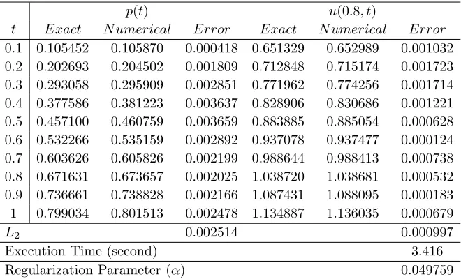
The results obtained for u(0, t) = p(t) and u(0.8, t) with k = 0.001, h = 0.1 and
β = 0.5 with noisy data (noisy data=input data+(0.0001) rand(1)) are presented in Table1and Figures1,2.
Table 1. The comparison between exact solution and numerical
so-lution for p(t) with the noisy data by using cubic B-spline method and Tikhonov2nd whenβ= 0.5 for Example 7.1.
p(t) u(0.8, t)
t Exact N umerical Error Exact N umerical Error
0.1 0.105452 0.105870 0.000418 0.651329 0.652989 0.001032 0.2 0.202693 0.204502 0.001809 0.712848 0.715174 0.001723 0.3 0.293058 0.295909 0.002851 0.771962 0.774256 0.001714 0.4 0.377586 0.381223 0.003637 0.828906 0.830686 0.001221 0.5 0.457100 0.460759 0.003659 0.883885 0.885054 0.000628 0.6 0.532266 0.535159 0.002892 0.937078 0.937477 0.000124 0.7 0.603626 0.605826 0.002199 0.988644 0.988413 0.000738 0.8 0.671631 0.673657 0.002025 1.038720 1.038681 0.000532 0.9 0.736661 0.738828 0.002166 1.087431 1.088095 0.000183 1 0.799034 0.801513 0.002478 1.134887 1.136035 0.000679
L2 0.002514 0.000997
Execution Time (second) 3.416
Figure 1. The plots of approximate solution, exact solution and
absolute error ofp(t) for Example7.1with the noisy data.
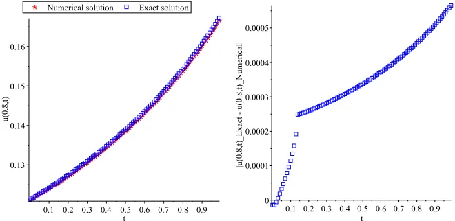
Figure 2. The plots of approximate solution, exact solution and
absolute error ofu(0.8, t) for Example7.1with the noisy data.
Example 7.2. In this example, consider the following inverse problem:
with given data
u(x,0) = 1
3arcsinh(
x+ 0.25
2√2 ),
u(1, t) = 1
3arcsinh( 1.25 2√2−t),
u(0.5, t) =1
3arcsinh( 0.75
2√2−t).
The exact solutions in a closed form are given by
u(x, t) =1
3arcsinh(
x+ 0.25 2√2−t).
For numerical computation, we take withβ = 0.5,k= 0.001 andh= 0.1 for estimate
u(0, t) =p(t) andu(0.8, t) with noisy data (noisy data=input data+(0.0001) rand(1)) and results are reported in Table2and Figures 3,4.
Table 2. The comparison between exact solution and numerical
so-lution for p(t) with the noisy data by using cubic B-spline method and Tikhonov2nd whenβ= 0.5 for Example 7.2.
p(t) u(0.8, t)
t Exact N umerical Error Exact N umerical Error
0.1 0.030186 0.032651 0.002464 0.124042 0.123961 0.000112 0.2 0.031011 0.034422 0.003411 0.127285 0.127061 0.000258 0.3 0.031908 0.035575 0.003667 0.130797 0.130553 0.000281 0.4 0.032887 0.036842 0.003955 0.134617 0.134350 0.000307 0.5 0.033961 0.038248 0.004286 0.138794 0.138501 0.000336 0.6 0.035149 0.039820 0.004670 0.143386 0.143064 0.000370 0.7 0.036471 0.041591 0.005120 0.148468 0.148112 0.000409 0.8 0.037954 0.043607 0.005653 0.154134 0.153739 0.000454 0.9 0.039634 0.045926 0.006292 0.160505 0.160065 0.000507 1 0.041558 0.048628 0.007069 0.167743 0.167249 0.000570
L2 0.004577 0.0003608
Execution Time (second) 5.632
Figure 3. The plots of approximate solution, exact solution and
absolute error ofp(t) for Example7.2with the noisy data.
Figure 4. The plots of approximate solution, exact solution and
absolute error ofu(0.8, t) for Example7.2with the noisy data.
Example 7.3. We consider the following inverse problem
with given data
u(x,0) = (2−0.5x)14,
u(1, t) = ( 0.5
t+ 1 + 1 8
ln(t+ 1) (t+ 1) + 1)
1 4,
u(0.5, t) = ( 1.5 2t+ 2 +
1 8
ln(t+ 1) (t+ 1) + 1)
1 4.
The exact solution of this problem is
u(x, t) = (2−x 2t+ 2 +
1 8
ln(t+ 1) (t+ 1) + 1)
1 4,
For numerical computation, we take withβ = 0.5,k= 0.001 andh= 0.1 for estimate
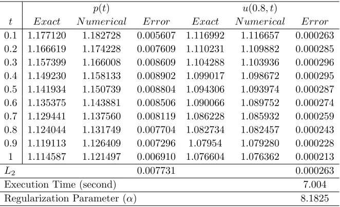
u(0, t) = p(t) and u(0.8, t) with noisy data and results are reported in Table 3 and Figures5,6.
Table 3. The comparison between exact solution and numerical
so-lution for p(t) with the noisy data by using cubic B-spline method and Tikhonov2nd whenβ= 0.5 for Example 7.3.
p(t) u(0.8, t)
t Exact N umerical Error Exact N umerical Error
0.1 1.177120 1.182728 0.005607 1.116992 1.116657 0.000263 0.2 1.166619 1.174228 0.007609 1.110231 1.109882 0.000285 0.3 1.157399 1.166008 0.008609 1.104288 1.103936 0.000296 0.4 1.149230 1.158133 0.008902 1.099017 1.098672 0.000295 0.5 1.141934 1.150739 0.008804 1.094306 1.093974 0.000287 0.6 1.135375 1.143881 0.008506 1.090066 1.089752 0.000274 0.7 1.129441 1.137560 0.008119 1.086228 1.085932 0.000259 0.8 1.124044 1.131749 0.007704 1.082734 1.082457 0.000243 0.9 1.119113 1.126409 0.007296 1.07954 1.079280 0.000228 1 1.114587 1.121497 0.006910 1.076604 1.076362 0.000213
L2 0.007731 0.000263
Execution Time (second) 7.004
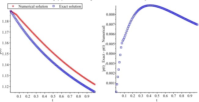
Figure 5. The plots of approximate solution, exact solution and
absolute error ofp(t) for Example7.3with the noisy data.
Figure 6. The plots of approximate solution, exact solution and
absolute error ofu(0.8, t) for Example7.3with the noisy data.
8. Conclusion
A numerical method, to estimate unknown boundary conditions is proposed and the following results are obtained.
• The present study successfully applies the numerical method to inverse prob-lems.
extra effort to deal with the nonlinear terms. Therefore, the equations are solved easily and elegantly using the present method.
• Numerical examples also verified the efficiency and accuracy of the method that can be obtained within a couple of minutes CPU time at Core(i5)–2.67 GHz PC.
• The present method has been found stable with respect to small perturbation in the input data.
References
[1] R. C. Aster, B. Borchers, and C. Thurber,Parameter estimation and inverse problems. Text-book, New Mexico, Tech., 2003.
[2] F. Auricchio, L. Beirao da Veiga, T. Hughes, A. Reali, and G. Sangalli,Isogeometric collocation methods,Mathematical Models and Methods in Applied Sciences,20(11) (2010), 2075–2107. [3] J. R. Cannon, Determination of an unknown heat source from overspecified boundary data,
SIAM J. Numer. Anal.,5(2) (1968), 275–286.
[4] J. R. Cannon, Y. Lin, and S. Wang,Determination of a control parameter in a parabolic partial differential equation,J. Aust. Math. Soc. Ser. B,33(1991), 149–163.
[5] M. Dehghan,An inverse problem of finding a source parameter in a semilinear parabolic equa-tion,Appl. Math. Model.,25(2001), 743–754.
[6] M. Dehghan, parameter determination in partial differential equation from the overspecified data,Math. Comput. Model.,41(23) (2005), 196–213.
[7] M. Dehghan and M. Lakestani, The Use of cubic B-spline scaling functions for solving the one-dimensional hyperbolic equation with a nonlocal conservation condition,Numer. Methods Partial Differential Eq.,23(6) (2007), 1277–1289.
[8] M. Dehghan, S. A. Yousefi, and K. Rashdi,Ritz-Galerkin method for solving an inverse heat conduction problem with a nonlinear source term via Bernstein multi-scaling functions and cubic B-spline functions,Inverse Prob. Sci. Eng.,21(2013), 500–523.
[9] L. Elden, A note on the computation of the generalized cross-validation function for ill-conditioned least squares problems,BIT,24(1984), 467–472.
[10] K. Eric Chu,Singular Value and Generalized Singular Value Decompositions and the Solution of Linear Matrix Equations,Linear Algebra and its Applications,88(1987), 83–98.
[11] A. G. Fatullayev and S. Cula,An iterative procedure for determining an unknown spacewise-dependent coeifficient in a parabolic equation,Appl. Math. Lett.,22(2009), 1033–1037. [12] S. Foadian, R. Pourgholi, and S. H. Tabasi,Cubic B-spline method for the solution of an inverse
parabolic system,Applicable Analysis,97(3) (2018), 438–465.
[13] G. H. Golub, M. Heath, and G. Wahba,Generalized cross-validation as a method for choosing a good ridge parameter,Technometrics,21(2) (1979), 215–223.
[14] H. Gomez and L. De Lorenzis,The variational collocation method,Computer Methods in Ap-plied Mechanics and Engineering,309(2016), 152–181.
[15] Y. C. Hon and T. Wei,A fundamental solution method for inverse heat conduction problem, Eng. Anal. Bound. Elem.,28(2004), 489–495.
[16] V. Isakov,Inverse Problems for Partial Differential Equations,Springer, New York, 1998. [17] M. K. Kadalbajoo, V. Gupta, and A. Awasthi,A uniformly convergent b-spline collocation
method on a nonuniform mesh for singularly perturbed one-dimensional time-dependent linear convection diffusion problem,Journal of Computational and Applied Mathematics,220(2008), 271–289.
[18] K. A. Khalid, K. R. Raslan, and T. S. El-Danaf,Non-polynomial Spline Method for Solving Coupled Burgers Equations,Comput. Methods Differ. Equ.,3(3) (2015), 218–230.
[20] L. Martin, L. Elliott, P. J. Heggs, D. B. Ingham, D. Lesnic, and X. Wen, Dual reciprocity boundary element method solution of the Cauchy problem for Helmholtz-type equations with variable coefficients,J. Sound Vib.,297(2006), 89–105.
[21] M. Montardini, G. Sangalli, and L. Tamellini, Optimal-order isogeometric collocation at Galerkin superconvergent points,Computer Methods in Applied Mechanics and Engineering, 316(2017), 741–757
[22] R. Pourgholi, N. Azizi, Y. S. Gasimov, F. Aliev, and H. K. Khalafi,Removal of numerical instability in the solution of an inverse heat conduction problem, Commun. Nonlinear Sci. Numer. Simul.,14(6) (2009), 2664–2669.
[23] R. Pourgholi, H. Dana, and S. H. Tabasi, Solving an inverse heat conduction problem using genetic algorithm: sequential and multi-core parallelization approach,Appl. Math. Modelling, 38(7) (2014), 1948–1958.
[24] R. Pourgholi and A. Saeedi,Applications of cubic B-splines collocation method for solving non-linear inverse parabolic partial differential equations,Numerical Methods for Partial Differential Equations,34(8) (2016), 1–17.
[25] A. G. Ramm, An inverse problem for the heat equation, J. Math. Anal. Appl., 264 (2004), 691–697.
[26] A. G. Ramm, Inverse problems,Springer, New York, 2005.
[27] W. Rudin,Principles of mathematical analysis,McGraw-Hill Inc., Third Edition, 1976. [28] D. Schillinger, J. A. Evans, A. Reali, M. Scott, and T. Hughes,Isogeometric collocation: cost
comparison with Galerkin methods and extension to adaptive hierarchical NURBS discretiza-tions,Computer Methods in Applied Mechanics and Engineering,267(2013), 170–232. [29] A. Shidfar, G. R. Karamali, and J. Damirchi, An inverse heat conduction problem with a
nonlinear source term,Nonlinear Anal.,65(2006), 615–621.
[30] G. D. Smith, Numerical solution of partial differential equation: finite difference method, Learendom Press, Oxford, 1978.