A new method for constructing exact solutions for a time-fractional
differential equation
Elham Lashkarian∗
Faculty of Mathematical Sciences, Shahrood University of Technology, Shahrood, Semnan, Iran.
E-mail: [email protected]
Seyed Reza Hejazi
Faculty of Mathematical Sciences, Shahrood University of Technology, Shahrood, Semnan, Iran.
E-mail: [email protected]
Noora Habibi
Faculty of Mathematical Sciences, Shahrood University of Technology, Shahrood, Semnan, Iran.
E-mail: [email protected]
Abstract In the present paper the process of finding new solutions from previous solutions of a given fractional differential equation (FDE) is considered. For this issue, first we should construct an exact solution by using the symmetry operators of the equation. Then, the commutator brackets of the obtained operators give new solutions from old ones via a systematic method.
Keywords. Lie point symmetry, Fractional calculus, Fractional differential equation, Exact solution.
2010 Mathematics Subject Classification. 76M60, 34K37, 34K06, 26A33.
1. Introduction
In the last decade FPDEs have attracted considerable interest. This kind of equa-tion plays an important role in various fields of sciences, for example engineering, elec-trochemistry, biology, economics, modeling, electronics, dynamics, and many other sciences [10, 12, 13]. Lie symmetries method have many efficient applications in physics and mathematics. As an important application of symmetry operators is the reduction procedure. This is possible from a similarity variable obtaining from the symmetry and Erdelyi-Kober. In this paper time FDE
Dαtu=xuxx+f(x)ux, (1.1)
is considere, whereDα
tuis the fractional derivative of orderα, 0< α≤1 andf(x)
is an arbitrary function.
Received: 25 December 2017 ; Accepted: 07 November 2018. ∗Corresponding author.
Firstly, we present the complete algebra of Lie point symmetries for Eq. (1.1). With the aid of calculated symmetries, Eq. (1.1) is reduced and a list of exact solutions are found [1, 2, 8,9]. The main goal of the paper is to build new solutions from the old ones by using the obtained exact solutions.
Some researches applied Lie group method for FDEs in the sense of the Caputo derivative and derived similarity solutions [4,11]. In this work, we give group classi-fication of Eq. (1.1), based on Riemann-Lioville derivative [5].
The organization of the paper sets in 6 sections; In section 2, we give some notations and preliminaries of equation with fractional order. The infinitesimal transformations and the determining equations of Lie symmetries are introduced in section 3. Section 4 is devoted to reduction precess for obtaining exact solutions of Eq. (1.1) in three separated cases. New exact solutions with the aid of obtained solutions, are presented in section 5. Finally, section 6 is dedicated to obtained results.
2. Fractional Calculus
There is no unique definition for fractional derivatives, such as modified Riemann-Liouville derivative, Grunwald-Letnikov derivative, Caputos, Riesz, Miller and Ross fractional derivative . Here we consider the most common definition named in Rie-mann and Liouvill derivative. In the sequel that, based on what is required in this work we give some basic definitions and properties of the fractional calculus theory [6]. Let us define
Dαtf(t) =
dnf
dtn α=n
dn dtnI
n−αf(t) 0≤n−1< α < n,
(2.1)
wheren∈N,Iβf(t) is the Riemann-Liouville fractional integral of orderβ , namely
Iβf(t) = 1 Γ(µ)
Z t
0
(t−s)(β−1)f(s)ds, β >0.
By definition, we haveI0f(t) =f(t) and it satisfies the stability propertyIν1 t I
ν2 t f(t) =
Iν1+ν2
t f(t) and Γ(ν) =
Z ∞
0
xν−1e−xdx, ν ∈R+, is the standard gamma function.
Definition 2.1. The Riemann-Liouville fractional partial derivative is defined by,
∂αtu(t, x) =
∂nu
∂tn α=n
1 Γ(n−α)
∂n
∂tn
Z t
0
(t−s)n−α−1u(s, x)ds 0≤n−1< α < n,
where∂n
t is the usual derivative of integer ordern.
The laplace transform of Riemann-Liouville fractional derivative of orderα >0 is [14]
L{Dαf(t)}=sαF(s)−
∞
X
k=0
sk{Dtα−k−1f(t)}t=0. (2.2)
whereL{f(t)}=F(s) =
Z ∞
0
e−stf(t)dt. A two-parameter function of Mittag-Leffler
type was defined by the series expansion [15]
Eα,β(z) =
∞
X
k=0
zk
Γ(αk+β), α, β∈C, Re(α)>0, Re(β)>0.
Some of the relationships are as follows:
Dν[tβ−1Eα,β(atα)] =tβ−ν−1Eα,β−ν(atα), ν >0, α >0, a∈R.
L{tαk+β−1Eα,β(k)(±atα)}= k!s
α−β
(sα∓a)k+1, Re(s)>|a|
1 α.
Definition 2.2. The Erdelyi-Kober fractional differential operator Pβτ,α of order α
is defined as [6]
Pβτ,αg:=
n−1 Y
j=0
τ+j− 1
βθ d dθ
Kβτ+α,n−αg(θ),
n=
[α] + 1 α /∈N
α α∈N,
where
Kβτ,αg:= (
1 Γ(α)
R∞ 1 (u−1)
α−1u−(τ+α)g(θuβ1)du α >0
g(θ) α= 0, (2.3)
is the Erdelyi-Kober fractional integral operator. Also we have
∂n ∂tn
h
tχ(Kβτ,n−αg)i(θ) = tχ−n
n−1 Y
j=0
χ−n+ 1 +j+aθd dθ
Kβχ−n+α+1,n−αg(θ)
= tχ−nPβχ−n+1,α(θ), (2.4)
if
t∂
∂tg(θ) =aθ d
dθg(θ), θ=xt
3. Symmetry analysis of FDEs.
Lie symmetries with the prolongation formula for FDEs have been given by Gazizov [3]. According to this method, Eq.FDE (1.1) is invariant under a one parameter continuous transformations with parameterε[16,17,18],
t∗=t+εξ0(t, x, u) +O(ε2), x∗=x+εξ1(t, x, u) +O(ε2),
u∗=u+εη(t, x, u) +O(ε2), ∂
αu∗
∂t∗ = ∂αu
∂tα +εζ
α,t(t, x, u) +O(ε2),
∂u∗ ∂x∗ =
∂u ∂x +εζ
x(t, x, u) +O(ε2), ∂ 2u∗
∂x∗2 =
∂2u ∂x2 +εζ
xx(t, x, u) +O(ε2),
(3.1)
where
ζx = Dxη−utDxξ0−uxDxξ1, ζxx=Dxζx−uxtDxξ0−uxxDxξ1,
ζα,t = ∂
αη
∂tα + (ηu−αDt(ξ
0))∂
αu
∂tα −u
∂αηu
∂tα −
∞ X n=1 α n
Dnt(ξ1)Dtα−n(ux)
+ ∞ X n=1 α n
∂nη u
∂tn −
α
n+ 1
Dnt+1(ξ0)
Dαt−n(u) +µ,
(3.2) and µ= ∞ X n=2 n X m=1 m X k=1
k−1 X r=0 α n n m k r 1 k!
tn−α
Γ(n−α+ 1)(−u)
r∂ m
∂tm(u k−r) ∂
n−m+k
∂tn−m∂uk,
also αn= Γ(n+1)Γ(Γ(α+1)α+1−n).
HereDx denotes total derivative operator defined by:
Dx=
∂ ∂x+ux
∂ ∂u+uxx
∂ ∂ux
+. . . .
If
X =ξ0∂ ∂t +ξ
1 ∂
∂x +η ∂
∂u, (3.3)
be a symmetry operator for the Eq. (1.1), which is known in the literature as an infinitesimal operator or generator of the groupG, we must have
ξ0= dt
∗
dε|ε=0 ξ
1= dx∗
dε |ε=0 η = du∗
dε |ε=0.
According to the infinitesimal invariance criterion, Eq. (1.1) admits transformation group (3) if the prolonged vector field Pr(α,2)X annihilates (1.1) on its solution, namely,
The operator Pr(α,2)X takes the form:
Pr(α,2)X=X+ζα,t∂∂α tu+ζ
x∂ ux+ζ
xx∂ uxx,
whereζxand ζxx are defined in (3.2). Now, we will investigate the invariance
prop-erties of the time fractional Eq. (1.1). The invariance criterion takes the form
ζα,t−(uxx+f0(x)ux)ξ1−f(x)ζx−xζxx= 0. (3.4)
Solving (3.4) along with (3.2), we derive the following characteristic system:
ξt1=ξ
0
u=ξ
1
u=ξ
0
x=ηuu= 0,
xηu−αxξt0−ξ
1
−x(ηu−2ξx1) = 0,
−αf(x)ξt0−f0(x)ξ1+f(x)ξx1−x(2ηxu−ξxx1 ) = 0,
∂αtη−u∂αtηu−f(x)ηx−xηxx= 0,
α n
∂tnηu−
α n+ 1
Dnt+1ξ0= 0.
With classification of solution of this system, we obtain solution of Eq. (1.1), for arbitraryf(x) andα∈(0,1], such as
ξ0=c1t+c2, ξ1=αc1x+c3 √
x, η =F1(x)u+F2(t, x),
wherec1, c2 andc3 are arbitrary constants.
For three cases we obtain different symmetries for Eq. (1.1). • Forβ =f(x) =12, Eq. (1.1) translates to:
Dαtu=xuxx+
1
2ux. (3.5)
The Lie symmetries of Eq. (3.5) are found as follows:
X1=αx
∂ ∂x+t
∂
∂t, X2=
√
x ∂
∂x, X3=
∂ ∂t,
X4=u
∂
∂u, XF2=F2(t, x)
∂
∂u. (3.6)
• Forβ =f(x) =32, we have
Dαtu=xuxx+
3
2ux, (3.7)
with Lie symmetries,
X1=αx
∂ ∂x+t
∂
∂t, X3=
∂
∂t, X4=u
∂ ∂u,
X5= √
x ∂ ∂x−
1 2√xu
∂
∂u, XF2 =F2(t, x)
∂
∂u. (3.8)
• Forβ =f(x) = 1+3
√
x
2(1+√x), the Eq. (1.1) turns to
Dαtu=xuxx+
1 + 3√x
with following symmetries:
X3=
∂
∂t, X4=u
∂
∂u, X6=αx
∂ ∂x+t
∂ ∂t+
α
2(1 +√x)u
∂ ∂u,
X7= √
x∂
∂x −
1 2(1 +√x)u
∂
∂u, XF2 =F2(t, x)
∂
∂u. (3.10)
4. Exact Solutions or Reduction equations by using Lie method
In this section we give some exact solutions for Eq. (3.5). • At first, we consider the symmetry X1 = αx∂x∂ +t
∂
∂t, the corresponding
characteristic equation is of the form:
dx
αx =
dt
t =
du
0 . (4.1)
Integration of (4.1) provides the following similarity function
u=g(t, x) =g(θ) =g(xt−α).
Letn−α < α < n,n= 1,2,3, . . ..
According to the Riemann-Liouville fractional derivative, once we get:
∂αu
∂tα =
∂ ∂tn
1 Γ(n−α)
Z t
0
(t−s)n−α−1g(xs−2α)ds
, (4.2)
Letν = st, we have ds=−t
ν2dν. So the above statement can be expressed
as:
∂αu
∂tα =
∂ ∂tn
1 Γ(n−α)
Z t
0
tn−αν−(n−α+1)(ν−1)n−α−1g(θνα)dν
= ∂
∂tn
h
tn−αK12,n−α α
g(θ)i
= t−α
n−1 Y
j=0
1−α+j+θ d dθ
K11,n−α α
g(θ)
= t−αP11−α,α α
g(θ). (4.3)
By substituting the solutionu=g(xt−2α) into FPDE (3.5), one can get:
∂αu
∂tα =xuxx+
1 2ux=t
−α(θg ξξ+
1
2gξ). (4.4) Thus, the time fractional equation (3.5) can be reduced into an FODE:
P11−α,α α
g(θ) =θg00+1 2g
0. (4.5)
• ForX2= √
x∂x∂ , with substituting u=g(t) in Eq. ( 3.5) we have ∂∂tααg = 0 .
So with the aid of Laplace transformation (2.2) we obtaing(t) = (αtα−−1)!1 . • ForX3 = ∂t∂, by using u=g(x) and placing it in Eq. (3.5), we havexg00+
1 2g
0= 0. Sog(x) =c
1+c2 √
xis a solution of Eq. (3.5).
Other solutions under symmetries X1+X4, X2+X4 and X3+X4 are summerized in Table (1), whereA= 2pxt−αe−tE
Table 1. Results For FDE (3.5)
Symmetries Exact Solutions Reduced equations
X1 u=g(xt−α) =g(θ)
P11−α,α α
g(θ) =θg00+12g0.
X2 u= t
α−1
Γ(α)
X3 u=c1+c2
√
x
X1+X4 u=tg(xt−α) =tg(θ)
P21−α,α α
g(θ) =θg00+12g0.
X2+X4 u=e2
√
xtα−1E
α,α(tα)
X3+X4 u=et[c1sinh(A) +c2cosh(A)]
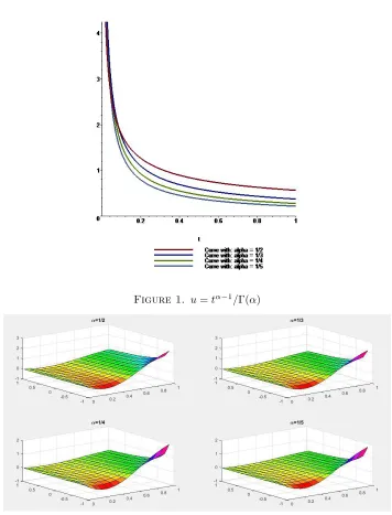
The exact solutions of Eq. (3.7) and (3.9) are given in Tables (2) and (3) respectively. Graph of solutions are shown in Figure 1, 2, 3 and 4 too.
Table 2. Results For FDE (3.7)
Symmetries Exact Solutions Reduced equations
X1 u=g(xt−α) =g(θ)
P11−α,α α
g(θ) =
θg00+32g0.
X3 u=c1+√c2x
X5 u= √1xt
α−1
Γ(α)
X3+X4 u= e
t
√
x[c1sinh(A) +c2cosh(A)]
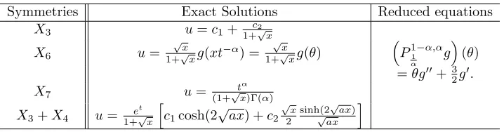
Table 3. Results For FDE (3.9)
Symmetries Exact Solutions Reduced equations
X3 u=c1+1+c√2x
X6 u=
√
x
1+√xg(xt
−α) = √x
1+√xg(θ)
P11−α,α α
g(θ)
=θg00+3 2g
0.
X7 u= t
α
(1+√x)Γ(α)
X3+X4 u= e
t
1+√x
h
c1cosh(2 √
ax) +c2
√
x
2
sinh(2√ax)
√
ax
i
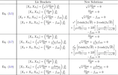
5. New solutions obtaining from old ones
form of XF2. This provides a route to the generation of new similarity solutions
associated toXi. The structure of the new solutions constructed from Lie brackets
of the symmetries are coming in Table4withB = q
xΓ(Γ(−α,tα)).
Table 4. New solutions
Lie Brackets New Solutions
[X2, XF2] =
√
x∂fold ∂x
∂ ∂u
√
x∂fold ∂x = 0
Eq. (3.5) [X3, XF2] =
∂f old ∂t ∂ ∂u ∂fold ∂t = 0
[X2+X4, XF2] =
√
x∂fold ∂x −fold
∂ ∂u
√
x∂fold
∂x −fold= 0
[X3+X4, XF2] =
∂f
old ∂t −fold
∂
∂u e
th2 sinh(2√B) + 2 cosh(2√B)i
×h xe−t
t1+αΓ(−α)+ 2B
i h
xe−t
2t1+αΓ(−α)√B
i
−fold= 0
[X3, XF2] =
∂f old ∂t ∂ ∂u ∂fold ∂t = 0
Eq. (3.7) [X5, XF2] =
√
x∂fold ∂x +
1 2√xfold
∂ ∂u
√
x∂fold ∂x +
1
2√xfold= 0
[X3+X4, XF2] =
∂f
old ∂t −fold
∂ ∂u et √ x h
2 sinh(2√B) + 2 cosh(2√B)i
×h xe−t
t1+αΓ(−α)+ 2B
i h
xe−t
2t1+αΓ(−α)√B
i
−fold= 0
[X3, XF2] =
∂fold ∂t ∂ ∂u ∂fold ∂t = 0
Eq. (3.9) [X7, XF2] =
√
x∂fold ∂x +
fold
2(1+√x)
∂ ∂u
√
x∂fold ∂x +
fold
2(1+√x) = 0 [X3+X4, XF2] =
∂f
old ∂t −fold
∂ ∂u
∂fold
∂t −fold= 0
6. Conclusion
Figure 1. u=tα−1/Γ(α)
Figure 2. u=√1
x tα−1
Figure 3. u= √et
x[sinh(A) + cosh(A)]
Figure 4. u= t α
References
[1] V. D. Djordjevica and T. M. Atanackovic, Similarity solutions to nonlinear heat conduction and Burgers/Korteweg-deVries fractional equations, Journal of Computational and Applied Mathematics,222(2) (2008), 701-714.
[2] R. K. Gazizov, A. A. Kasatkin, and S. Y. Lukashchuk,Group-invariant solutions of fractional differential equations, In: Machado J., Luo A., Barbosa R., Silva M., Figueiredo L. (eds) Non-linear Science and Complexity. Springer, Dordrecht, 2011.
[3] R. Gazizov, A. Kasatkin, and S. Y. Lukashchuk, Symmetry properties of fractional diffusion equations, Physica Scripta,T136(2009), 014016 (5pp).
[4] W. Guo-Cheng,Lie Group Classifications and Non-differentiable Solutions for Time-Fractional Burgers Equation, Communications in Theoretical Physics,55(6) (2011), 1073-1076.
[5] G. Jumarie,Modified Riemann-Liouville derivative and fractional Taylor series of nondifferen-tiable functions further results, Computers and Mathematics with Applications,51(9-10) (2006), 1367-1376.
[6] V. Kiryakova,Generalized fractional calculus and applications, Pitman Research Notes in Math-ematics, 301, Longman1994.
[7] R. J. Knops and C. A. Stuart,Quasiconvexity and uniqueness of equilibrium solutions in non-linear elasticity, Archive for Rational Mechanics and Analysis,86(3) (1984), 233-249.
[8] E. Lashkarian and S. R. Hejazi,Polynomial and non-polynomial solutions set for wave equation using Lie point symmetries, Computational Methods for Differential Equations,4(4) (2016), 298-308.
[9] H. Liu, Complete group classifications and symmetry reductions of the fractional fifth-order KdV types of equations, Studies in Applied Mathematics,131(4) (2013), 317-330.
[10] R. L. Magin,Fractional calculus models of complex dynamics in biological tissues, Computers and Mathematics with Applications,59(5) (2010), 1586-1593.
[11] A. B. Malinowska, M. R. S. Ammi, and D. F. M. Torres,Composition Functionals in Fractional Calculus of Variations, arXiv:1009.3883.
[12] K. S. Millera and B. Ross,An Introduction to the Fractional Integrals and Derivatives-Theory and Applications, John Willey and Sons, New York 1993.
[13] F. C. Meral, T.J. Royston, and R.Magin,Fractional calculus in viscoelasticity: An experimental study, Communications in Nonlinear Science and Numerical Simulation,15(4) (2010), 939-945. [14] I. Podlubny,Fractional Differential Equations: An Introduction to Fractional Derivatives, Frac-tional Differential Equations, to Methods of Their Solution and Some of Their Applications, Academic Press, 1999.
[15] H. J. Seybold and R. Hilfer,Numerical results for the generalized Mittag-Leffler function, Frac-tional Calculus and Applied Analysis ,8(2005), 127-39 .
[16] G. Wang and T. Xu,Symmetry properties and explicit solutions of the nonlinear time fractional KDV equation Boundary Value Problems, Boundary Value Problems,232(2013), 1-13. [17] G. W. Wang, X. Q. Liu, and Ying-yuan Zhang,Lie symmetry analysis to the time fractional
generalized fifth-order KDV equation, Communications in Nonlinear Science and Numerical Simulation,18(9) (2013), 2321-2326.
![Figure 3. u =√etx [sinh(A) + cosh(A)]](https://thumb-us.123doks.com/thumbv2/123dok_us/8943180.1852548/10.612.132.482.114.296/figure-u-etx-sinh-a-cosh-a.webp)
