DEMOGRAPHIC RESEARCH
VOLUME 30, ARTICLE 62, PAGES 1681–1696
PUBLISHED 28 MAY 2014
http://www.demographic-research.org/Volumes/Vol30/62/ DOI: 10.4054/DemRes.2014.30.62
Research Article
A note on computing average state occupation
times
Jan Beyersmann
Hein Putter
This publication is part of the Special Collection on “Multistate Event History Analysis,” organized by Guest Editors Frans Willekens and Hein Putter.
c
2014 Jan Beyersmann & Hein Putter.
2 The relation between transition hazards and transition
probabilities 1682
3 Estimating expected waiting times 1685
4 Illustration 1686
5 Closing remarks 1691
A note on computing average state occupation times
Jan Beyersmann1
Hein Putter2
Abstract
OBJECTIVE
This review discusses how biometricians would probably compute or estimate expected waiting times, if they had the data.
METHODS
Our framework is a time-inhomogeneous Markov multistate model, where all transition hazards are allowed to be time-varying. We assume that the cumulative transition haz-ards are given. That is, they are either known, as in a simulation, determined by expert guesses, or obtained via some method of statistical estimation. Our basic tool is product integration, which transforms the transition hazards into the matrix of transition probabil-ities. Product integration enjoys a rich mathematical theory, which has successfully been used to study probabilistic and statistical aspects of multistate models. Our emphasis will be on practical implementation of product integration, which allows us to numerically ap-proximate the transition probabilities. Average state occupation times and other quantities of interest may then be derived from the transition probabilities.
1Ulm University, Germany. E-Mail: [email protected].
1.
Introduction
This review is motivated by an interdisciplinary workshop on ‘Multistate event history analysis’ at the Netherlands Interdisciplinary Demographic Institute, The Hague, in April 2011. The workshop brought together demographers and biometricians, who both use multistate models, but appear to follow somewhat different methodological traditions.
At the workshop, there were discussions on how to compute average state occupation times. The organizer, Frans Willekens, informed us that the most common approaches in demography use either piecewise linear approximations of the survival function or piece-wise constant transition hazards (personal communication). See also Gill and Keilman (1990) on these approaches, including a critique of the former method.
We review how biometricians might compute expected waiting times, if they had the data. In biometry, the restriction is that right-censoring typically precludes evaluating waiting time distributions on the whole of their support. In other words, the maximum follow-up in most of the data sets analyzed by biometricians is considerably smaller than the assumed maximum age in the population under study. As a consequence, it is more common to consider median waiting times (e.g., Brookmeyer and Crowley 1982) or expectations restricted to a maximum follow-up (e.g., Andersen et al. 1993, Example IV.3.8). In the context of demography, expected (restricted) waiting times are arguably more relevant, for instance for policy making.
The key idea is that a certain transformation, product integration, allows us to move from the transition hazards of a time-inhomogeneous Markov process to the matrix of transition probabilities. As also noted by Gill and Keilman (1990), combined with the initial distribution of the process, this allows us to derive expected waiting times in a given state and other quantities of interest.
In demography, product integration appears to be rarely used. Gill and Keilman (1990) mention the relation, but then proceed to attack a different problem, namely estimation of constant transition hazards with population registry data. In a recent tutorial on multistate methods, Kuo, Suchindran, and Koo (2008) value product integration as a ‘basic tool’, but argue that it ‘is difficult to implement.’ These authors therefore proceed to work under special assumptions such as uniform right-censoring. Another reference is Schoen (2005) who mentions product integration as a tool for numerical evaluation, but then concentrates on special cases with an analytical solution.
2.
The relation between transition hazards and transition
probabilities
Consider a time-inhomogeneous Markov process(Xt)t≥0with state space{0,1,2, . . . , J}.
transition times. That is, if the process moves from statejto statek,j 6=k, at timet0, Xt0 =kandXt0−=j. HereXt0−refers to the state occupied by the process just before
timet0. We also assume that on any finite interval there are only finitely many
transi-tions. No assumptions are made on irreversibility of the multistate model. The Markov assumption is
P(Xt=k|Xs=j) = P(Xt=k|Xs=j,Past), s≤t, (1)
where we have written ‘Past’ for the history generated by the process. More formally, it is a sigma-algebra and, at times, reflects knowledge of the development of the process in the interval[0, s]. The Markov assumption states that the past and future of the process are independent, given the present. We will briefly discuss non-Markov processes in Section 5.
The matrix of transition probabilities is
P(s, t) := (Pjk(s, t))j,k, j, k∈ {0,1,2, . . . , J}, (2)
with transition probabilities
Pjk(s, t) := P(Xt=k|Xs=j), s≤t. (3)
Multiplying the initial distribution(P(X0= 0),P(X0= 1), . . . ,P(X0=J))of the
mul-tistate process withP(0, t)yields the state occupation probabilities(P(Xt= 0),P(Xt=
1), . . . ,P(Xt = J))at timet. These can, e.g., be used to compute the expected time
spent in statekas
Ek=
Z ∞
0
P(Xu=k) du, (4)
see, e.g., Equation (6) of Gill and Keilman (1990). The restricted expected time spent in statekis
Ekτ =
Z τ
0
P(Xu=k) du, (5)
whereτ is some fixed value, representing end of follow-up or some lower relevant time limit. In the Markov case, one can also define the expected remaining time (residual life expectancy) spent in statek, given that the subject is in statejat times, as
Ejks,τ =
Z τ
s
P(Xu=k|Xs=j) du, (6)
for τ ≤ ∞. For τ < ∞, this is a restricted expected remaining time spent in state
probabilities may be step functions which allow us to further simplify (4) and (5). We return to this issue later.
The aim is now to find the connection betweenP(s, t)and the cumulative transi-tion hazards (or intensities)Ajk(s),j 6= k, which we assume to be given. That is, the Ajk’s may have been pre-specified as in a simulation, determined by expert guesses or
statistically estimated. We writeAjj(t) = −P J
k=0,k6=jAjk(t)and we assume that Ajj(t)−Ajj(t−) ≥ −1. For the discrete case, the latter assumption is implied by the
fact that the probability of leaving statejat timet, on the condition that one is in statej
at the last time point beforet, does not exceed1. In the purely continuous case, we have
Ajj(t)−Ajj(t−) = 0. Our presentation below is indebted to Aalen and Johansen (1978)
and Gill and Johansen (1990), see also the textbook accounts in Andersen et al. (1993) and Aalen, Borgan, and Gjessing (2008).
Consider timess < v < t. Using the Markov property, we get for the(j, k)-th entry ofP(s, t)that
P(Xt=k|Xs=j) = J
X
˜ =0
P(Xv= ˜|Xs=j)·P(Xt=k|Xv= ˜). (7)
Ifvis close tot, the usual interpretation of the transition hazards is that
P(Xt=k|Xv= ˜)≈∆A˜k(t),˜6=k,
and consequently
P(Xt= ˜|Xv= ˜)≈1 + ∆A˜˜(t),
where∆Ak˜(t)isAk˜ (t)−A˜k(v). We summarize this by
P(Xt=k|Xs=j)≈ J
X
˜ =0
P(Xv= ˜|Xs=j)·(1(˜=k) + ∆Ak˜(t)), (8)
where we have written1(·)for the indicator function. The matrix version of (8) is
P(s, t)≈P(s, v) (I+ ∆A(t)), (9)
where we have writtenIfor the(J + 1)×(J + 1) identity matrix and∆A(t) is the (J+ 1)×(J+ 1)matrix with(j, k)entry∆Ajk(t).
Going through the approximation of (9) recursively and for a fine partitions=t0< t1< t2< . . . < tL−1< tL=tof the time interval[s, t], we get the approximation
P(s, t)≈ L
Y
l=1
We note two important facts about (10): First, the approximation is precisely what we need in order to numerically computeP(s, t). Secondly, the right hand side of (10) re-turns a step function which simplifies evaluating (4). (Note that for constant or piecewise constant transition intensities, explicit matrix exponential solutions of the product inte-gral are available (e.g. Andersen and Pohar Perme 2008); this is a well known result for homogeneous Markov processes (e.g. Kijima 1997). For practical implementation, these explicit solutions will also rely on some approximation, typically based on a Taylor ex-pansion.)
The mathematical task is now to show that the right hand side of (10) in fact ap-proachesP(s, t)for ever finer partitions of [s, t]. A complete account of this has been given by Gill and Johansen (1990). These authors suggest the followingproduct integral
notation for the limit of the finite product in (10),
u∈(s,t]
(I+ dA(u)), (11)
and they prove that the product integral (11) equalsP(s, t). In summary,
lim
max|tl−tl−1→0|
Y
(I+ ∆A(tl)) =
u∈(s,t]
(I+ dA(u)) =P(s, t). (12)
3.
Estimating expected waiting times
Combining relations (4)–(6) and (11) gives a relation between the transition intensities and the expected time spent in a given state. An estimate ofEk immediately presents
itself from these relations, namely
ˆ
Ek=
Z ∞
0
ˆ
P(Xu=k) du, (13)
whereP(ˆ Xu =k)would be obtained from estimates of the initial distribution( ˆP(X0 =
0),P(ˆ X0= 1), . . . ,P(ˆ X0=J))andPˆ(s, t)through estimatesAˆjk(s)of the cumulative
asymptotic unbiasedness using the continuous mapping theorem and to show correctness of the bootstrap for quantifying uncertainty using the functional delta method; we will dis-cuss the latter at the end of Section 5. Similar ‘plug in’ estimates have been used by, e.g., Lièvre, Brouard, and Heathcote (2003) and Touraine, Helmer, and Joly (2013). Dropping the statistical perspective, we note that researchers have also used the trapezoidal rule or the related, but more complex Simpson’s rule (also known asKeplersche Fassregel) for numerically approximating the integral in question. We do not consider these approaches here, but refer to Gill and Keilman (1990) who prove that using the trapezoidal rule may lead to implicit violations of the Markov assumption.
It is common for the cumulative transition intensities to be estimated as step-functions, for instance, using non-parametric methods such as the Nelson-Aalen estimate or using semi-parametric methods such as the Cox model or additive hazards. Then for a fixed statek,P(ˆ Xu =k)will be constant with respect touover time intervals. Suppose that
the values ofP(ˆ Xu=k)arepˆlon intervals[al−1, al)forl= 1, . . . , Lwitha0 = 0and aL = ∞. BothL, the seriesa0, . . . , aL andpˆ0, . . . ,pˆL may depend on the statek of
interest. ThenEˆk can be written as
ˆ
Ek = L
X
l=1
(al−al−1)ˆpl, (14)
which is both easy and quick to calculate. IfpˆL= 0, this sum is finite and the last element
of the sum is zero (and hence could be removed). IfpˆL >0, thenEˆkwill be infinite. In
that case it is appropriate to consider instead the restricted expected timeEτ
k spent in state kfrom Equation (5). An estimate ofEτ
k would then also be given by the right-hand side
of (14), the only difference with the unrestrictedEˆkbeing that hereaL=τ.
We also note that estimation of (13) using non- or semi-parametric methods requires that the assumed maximum age in the population is part of the data. If this is not the case, estimation of the restricted quantityEkτwould be more appropriate, whereτis some fixed value, representing end of follow-up or some lower relevant time limit, as noted earlier. Alternatively, one might use parametric models such as constant or piecewise constant transition intensities, which would allow for extrapolation beyond the maximum time contained in the data.
We refer to the closing Section 5 for a discussion on how to estimate uncertainty.
4.
Illustration
Retire-ment Study (HRS, Juster and Suzman 1995). The AHEAD survey includes a nationally representative sample of initially non-institutionalized persons born before 1923, aged 70 and older in 1993. The present analysis uses only the non-Hispanic white subset; the time scale is age. Subjects were interviewed every two years. For the purpose of illustra-tion, the fact that the data are actually panel data, hence interval-censored, is conveniently ignored. Properly taking interval censoring into account will only affect the initial esti-mation of the transition intensities, not the subsequent calculation of the expected time spent in the different states; it is this last step that we wish to illustrate. We will further comment on interval-censoring in Section 5.
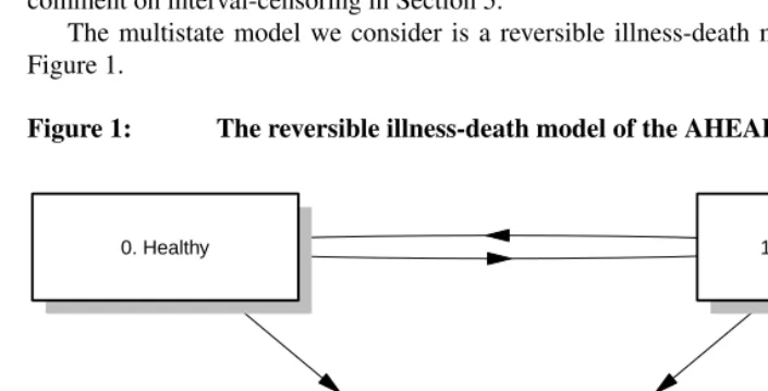
The multistate model we consider is a reversible illness-death model, illustrated in Figure 1.
Figure 1: The reversible illness-death model of the AHEAD data
0. Healthy 1. ADL disabled
2. Death
Figure 2 shows the estimated cumulative transition intensities for each of the four transitions, based on the non-parametric Nelson-Aalen estimates. They are shown for males (a) and females (b) separately.
Figure 2: Non-parametric estimates of the transition intensities in the US Health and Retirement Study, for males (a) and females (b) separately
75 80 85 90 95 100 105
0123456
Age
Cum
ulativ
e hazard
Healthy −> ADL disabled Healthy −> Death ADL disabled −> Healthy ADL disabled −> Death
Males
(a)
75 80 85 90 95 100 105
0123456
Age
Cum
ulativ
e hazard
Healthy −> ADL disabled Healthy −> Death ADL disabled −> Healthy ADL disabled −> Death
Females
(b)
The estimated transition intensities of disability (Healthy→ADL disabled) and re-covery (ADL disabled→Healthy), in gray, are comparable between males and females. The shape of the cumulative intensity of disability is convex, indicating that with older age the disability rate increases, while the shape of the cumulative intensity of recovery is concave, indicating a decreased recovery rate with older age. Death rates, in black, are considerably higher from the ADL disability state, compared to those from the healthy state. In a Cox proportional hazards model, the hazard ratio between the ADL disabled
→Death rate and the Healthy→Death rate was estimated as 2.89 (95% confidence inter-val (CI): 2.52 - 3.31) for males and 2.25 (95% CI: 1.99 – 2.55) for females. As expected, death rates are higher for males than for females.
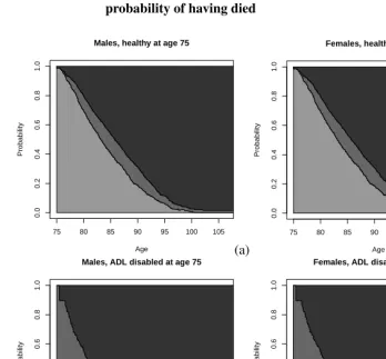
Figure 3 shows estimated transition probabilitiesPbjk(75, t)based on the transition
Figure 3: Stacked plots of estimated transition probabilitiesPbjk(75, t)for j = 0((a) and (b)), and forj = 1((c) and (d)). The lightest gray corresponds to the probability of being healthy, middle gray to the probability of being ADL disabled and the darkest gray to the probability of having died
75 80 85 90 95 100 105
0.0 0.2 0.4 0.6 0.8 1.0 Age Probability
Males, healthy at age 75
(a)
75 80 85 90 95 100 105
0.0 0.2 0.4 0.6 0.8 1.0 Age Probability
Females, healthy at age 75
(b)
75 80 85 90 95 100 105
0.0 0.2 0.4 0.6 0.8 1.0 Age Probability
Males, ADL disabled at age 75
(c)
75 80 85 90 95 100 105
0.0 0.2 0.4 0.6 0.8 1.0 Age Probability
Females, ADL disabled at age 75
(d)
Figure 3(a) and (b) show, for males and females respectively, estimates ofP0k(75, t),
upper curve isPb01(75, t), the probability of being ADL disabled, and finally the distance
between the upper curve and 1 isPb02(75, t), the death probability. Figure 3(c) and (d)
show estimates ofP1k(75, t), probabilities of being in statekat age t, given in state 1
(ADL disabled) at age 75. Clearly, until age 85 at least, the probability of being healthy at agetis much smaller in Figure 3(c) and (d), compared to Figure 3(a) and (b), and the probability of being ADL disabled much larger. Also the probability of having died is considerably larger in Figure 3(c) and (d), compared to Figure 3(a) and (b).
Estimates of the expected remaining time spent in a particular state can be “read off” from Figure 3 as the area between curves. For instance, for males, conditional on being healthy at age 75, an estimate of the expected remaining healthy life, Eb
75,τ 00 =
Rτ
75Pb00(75, u) du, is the area under thePb00(75, t)curve, i.e., the lightest gray area of
Figure 3(a). Similarly,Eb
75,τ 01 =
Rτ
75Pb01(75, u) duis the area between the lower and
up-per curve, the middle gray area of Figure 3(a). Both are easily calculated fromPb0k(75, t)
using the methods outlined in Section 3. Takingτ = 110, the expected remaining healthy life of males, given healthy at age 75 is estimated to be 9.21 years. For females this num-ber (the area under the lower curve of Figure 3(b)) is estimated as 10.04. Given subjects who are healthy at age 75, the expected remaining life spent in disability equals 2.26 years for males and 4.33 for females. Total remaining life for females (14.37 years) is almost three years longer than males (11.47), but more than two thirds of these additional years are spent in ADL disability.
Given subjects who are ADL disabled at age 75, expected remaining healthy life equals 2.63 years for males and 4.11 years for females; expected remaining life in dis-ability equals 5.21 years for males and 8.59 years for females. The difference between males and females in expected residual life is almost 5 years; again the majority of these additional life years is spent in disability.
5.
Closing remarks
Product integration is the mapping that switches from the transition hazards of a multistate model towards its matrix of transition probabilities. The product integral may easily be approximated by a finite product which allows us to evaluate expected waiting times and other quantities of interest even in the absence of closed formulae.
We refer to Gill and Johansen (1990) for a comprehensive overview on product in-tegration, including historic remarks. An important statistical paper is Aalen and Jo-hansen (1978), who used product integration on the matrix of the Nelson-Aalen estimators ofAjk(t). It is interesting to note that the resulting so-called Aalen-Johansen estimator
ofP(s, t), recently implemented in R by Allignol, Schumacher, and Beyersmann (2011) and de Wreede, Fiocco, and Putter (2011), may also be used for numerical approxima-tion. If the transition hazards have been determined for a simulation study, say, we may directly use the approximation of (10). Alternatively, we may simulate a large number of individuals, and subsequently compute the Aalen-Johansen estimator in order to approxi-mateP(s, t).
Important statistical papers following Aalen and Johansen (1978) include Gill and Jo-hansen (1990), who established compact differentiability of the product integral, which enables use of the function delta method; Andersen, Hansen, and Keiding (1991), who predicted transition probabilities based on Cox-type models for the transition hazards (re-cently made available in R by de Wreede, Fiocco, and Putter (2011)), and Aalen, Borgan, and Fekjær (2001), who used additive models for prediction.
stud-ied estimation of transition probabilities in Markov renewal models, also using product integration.
Throughout, our point of view has been that the transition hazards are given, i.e., known as in a simulation, determined by expert guesses or statistically estimated, and our aim has been to demonstrate the link from the transition hazards via the transition proba-bilities towards expected waiting times. In the illustration of Section 4, we have empha-sized this link, but have ignored that the data were interval-censored, a common compli-cation, not only with demographic data. One popular approach to account for interval-censoring are embedded Markov chains, see, e.g., Laditka and Wolf (1998), Izmirlian et al. (2000), Van Den Hout, Jagger, and Matthews (2009) and also Lièvre, Brouard, and Heathcote (2003), who have provided the popular IMaCh software (http://euroreves.ined. fr/imach/); see, e.g., Crimmins et al. (2009) and Cambois et al. (2011) for recent applica-tions of IMaCh. A recent review on statistical inference in the illness-death model without recovery in the presence of interval-censoring, has been given by Touraine, Helmer, and Joly (2013) who also pay special attention to life expectancies. In another recent pa-per, Wolf and Gill (2009) have compared using embedded Markov chains with ignoring interval-censoring; interestingly, these authors found that no method performed uniformly superior with respect to life expectancies.
References
Aalen, O., Borgan, Ø., and Fekjær, H. (2001). Covariate Adjustment of Event Histories Estimated from Markov Chains: The Additive Approach.Biometrics57(4): 993–1001.
doi:10.1111/j.0006-341X.2001.00993.x.
Aalen, O., Borgan, Ø., and Gjessing, H. (2008). Survival and Event History Analysis. New York: Springer.doi:10.1007/978-0-387-68560-1.
Aalen, O. and Johansen, S. (1978). An Empirical Transition Matrix for Non-homogeneous Markov Chains Based on Censored Observations.Scandinavian Journal of Statistics5: 141–150.
Allignol, A., Schumacher, M., and Beyersmann, J. (2011). Empirical Transition Matrix of Multi-State Models: The etm Package. Journal of Statistical Software38(4): 1–15.
http://www.jstatsoft.org/v38/i04/.
Allignol, A., Beyersmann, J., Gerds, T., and Latouche, A. (2013). A competing risks ap-proach for nonparametric estimation of transition probabilities in a non-Markov illness-death model. Lifetime Data Analysis.doi:10.1007/s10985-013-9269-1.
Andersen, P.K., Borgan, Ø., Gill, R., and Keiding, N. (1993). Statistical Models Based on Counting Processes. New York: Springer.doi:10.1007/978-1-4612-4348-9. Andersen, P.K., Hansen, L., and Keiding, N. (1991). Non-and Semi-Parametric
Estima-tion of TransiEstima-tion Probabilities from Censored ObservaEstima-tion of a Non-Homogeneous Markov Process.Scandinavian Journal of Statistics18: 153–167.
Andersen, P.K. and Pohar Perme, M. (2008). Inference for outcome probabilities in multi-state models.Lifetime Data Analysis14(4): 405–431.doi:10.1007/s10985-008-9097-x. Beyersmann, J., di Termini, S., and Pauly, M. (2013). Weak Convergence of the Wild Bootstrap for the Aalen-Johansen Estimator of the Cumulative Incidence Func-tion of a Competing Risk. Scandinavian Journal of Statistics 40(3): 387–402.
doi:10.1111/j.1467-9469.2012.00817.x.
Brookmeyer, R. and Crowley, J. (1982). A Confidence Interval for the Median Survival Time.Biometrics38(1): 29–41.doi:10.2307/2530286.
Cambois, E., Laborde, C., Romieu, I., and Robine, J.M. (2011). Occupational inequal-ities in health expectancies in France in the early 2000s: Unequal chances of reach-ing and livreach-ing retirement in good health. Demographic Research 25(12): 407–436.
doi:10.4054/DemRes.2011.25.12.
Change in Disability-Free Life Expectancy for Americans 70 Years Old and Older.
Demography46(3): 627–646.doi:10.1353/dem.0.0070.
Datta, S. and Satten, G.A. (2001). Validity of the Aalen-Johansen estimators of stage occupation probabilities and Nelson-Aalen estimators of integrated transition haz-ards for non-Markov models. Statistics & Probability Letters 55(4): 403–411.
doi:10.1016/S0167-7152(01)00155-9.
de Wreede, L.C., Fiocco, M., and Putter, H. (2011). mstate: An R Package for the Analy-sis of Competing Risks and Multi-State Models.Journal of Statistical Software38(7): 1–30.http://www.jstatsoft.org/v38/i07/.
Gill, R. and Keilman, N. (1990). On the estimation of multidimensional demographic models with population registration data.Mathematical Population Studies2(2): 119– 143.doi:10.1080/08898489009525298.
Gill, R.D. and Johansen, S. (1990). A Survey of Product-Integration with a View To-ward Application in Survival Analysis. The Annals of Statistics18(4): 1501–1555.
doi:10.1214/aos/1176347865.
Glidden, D.V. (2002). Robust Inference for Event Probabilities with Non-Markov Event Data.Biometrics58(2): 361–368. doi:10.1111/j.0006-341X.2002.00361.x.
Izmirlian, G., Brock, D., Ferrucci, L., and Phillips, C. (2000). Active Life Expectancy from Annual Follow-Up Data with Missing Responses. Biometrics56(1): 244–248.
doi:10.1111/j.0006-341X.2000.00244.x.
Juster, F.T. and Suzman, R. (1995). An Overview of the Health and Retirement Study.
The Journal of Human Resources30: S7–S56. doi:10.2307/146277.
Katz, S., Ford, A.B., Moskowitz, R.W., Jackson, B.A., and Jaffe, M.W. (1963). Studies of Illness in the Aged: The Index of ADL: A Standardized Mea-sure of Biological and Psychosocial Function. JAMA 185(12): 914–919.
doi:10.1001/jama.1963.03060120024016.
Kijima, M. (1997). Markov Processes for Stochastic Modeling. London: Chapman & Hall.doi:10.1007/978-1-4899-3132-0.
Kuo, T.M., Suchindran, C.M., and Koo, H.P. (2008). The multistate life table method: An application to contraceptive switching behavior. Demography 45(1): 157–171.
doi:10.1353/dem.2008.0013.
Laditka, S.B. and Wolf, D.A. (1998). New Methods for Analyzing
Ac-tive Life Expectancy. Journal of Aging and Health 10(2): 214–241.
Lièvre, A., Brouard, N., and Heathcote, C. (2003). The estimation of health expectancies from cross-longitudinal surveys. Mathematical Population Studies 10(4): 211–248.
doi:10.1080/713644739.
Martinussen, T. and Scheike, T. (2006). Dynamic Regression Models for Survival Data. New York: Springer.
Meira-Machado, L. and Pardinas, J. (2011). p3state.msm: Analyzing Survival Data from an Illness-Death Model. Journal of Statistical Software 38(3): 1–18.
http://www.jstatsoft.org/v38/i03.
Meira-Machado, L., Uña-Álvarez, J., and Cadarso-Suárez, C. (2006). Nonparametric estimation of transition probabilities in a non-Markov illness-death model. Lifetime Data Analysis12(3): 325–344. doi:10.1007/s10985-006-9009-x.
Schoen, R. (2005). Intrinsically dynamic population models. Demographic Research
12(3): 51–76. doi:10.4054/DemRes.2005.12.3.
Spitoni, C., Verduijn, M., and Putter, H. (2012). Estimation and Asymptotic Theory for Transition Probabilities in Markov Renewal Multi-State Models. The International Journal of Biostatistics8(1): 51–76.doi:10.1515/1557-4679.1375.
Touraine, C., Helmer, C., and Joly, P. (2013). Predictions in an illness-death model.
Statistical Methods in Medical Researchdoi:10.1177/0962280213489234.
Van Den Hout, A., Jagger, C., and Matthews, F.E. (2009). Estimating life expectancy in health and ill health by using a hidden Markov model. Journal of the Royal Sta-tistical Society: Series C (Applied Statistics) 58(4): 449–465. doi:10.1111/j.1467-9876.2008.00659.x.
van der Vaart, A. and Wellner, J.A. (1996). Weak Convergence and Empirical Processes. With Applications to Statistics. New York: Springer.