Volume 13 - Article 11 | Pages 231–280

in the population sciences published by the Max Planck Institute for Demographic Research Konrad-Zuse Str. 1, D-18057 Rostock · GERMANY www.demographic-research.org

DEMOGRAPHIC RESEARCH

VOLUME 13, ARTICLE 11, PAGES 231-280

PUBLISHED 17 NOVEMBER 2005

http://www.demographic-research.org/Volumes/Vol13/11/ DOI: 10.4054/DemRes.2005.13.11

Research Article

On the relationship between period and cohort

mortality

John R. Wilmoth

This article is part of Demographic Research Special Collection 4, “Human Mortality over Age, Time, Sex, and Place: The 1st _{HMD Symposium”.}

1 Introduction 232

2 Overview and fundamental concepts 233

2.1 Cohorts vs. periods 234

2.2 Quantum vs. tempo 234

2.3 Population dynamics vs. synthetic cohorts 234 2.4 Causes and consequences of partial (or surplus) quantum 236

2.5 Models of mortality change over time 238

3 Mortality functions and basic relationships 238

3.1 Single cohort model 238

3.2 Standard period-cohort model 240

3.3 Cohort distributions of age at death 242

4 Alternative measures of period mean lifespan 248 4.1

Relative size of a constant-birth population, e *0

249

4.2 _{Mean age at death in a constant-birth population,}

0

e′ 249

4.3

Tempo-adjusted life expectancy at birth, _eBF

0 or *e0

251

4.4 Comparison to period life expectancy at birth, e₀ 253

5 Trends in life expectancy at birth by period and cohort 255 5.1 Speed of change in historical trends 255 5.2 Intrinsic difference in period-cohort trends 257 5.3 Period-cohort trends in the linear shift model 258 5.4 Empirical application of the linear shift model 261

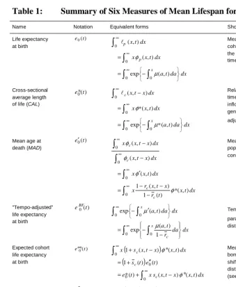
6 Comparison of six measures of mean lifespan 265

7 Conclusion 267

8 Acknowledgements 268

References 269

Appendix 271

A-1. Percentile slopes of cohort distributions of age at death 271

On the relationship between period and cohort mortality

John R. Wilmoth 1

Abstract

In this paper I explore the formal relationship between period and cohort mortality, focusing on a comparison of measures of mean lifespan. I consider not only the usual measures (life expectancy at birth for time periods and birth cohorts) but also some alternative measures that have been proposed recently.

I examine (and reject) the claim made by Bongaarts and Feeney that the level of period e is distorted, or biased, due to changes in the timing of mortality. I show that 0

their proposed alternative measure, called “tempo-adjusted” life expectancy, is exactly equivalent in its generalized form to a measure proposed by both Brouard and Guillot, the cross-sectional average length of life (or CAL), which substitutes cohort survival probabilities for their period counterparts in the calculation of mean lifespan. I conclude that this measure does not in any sense correct for a distortion in period life expectancy at birth, but rather offers an alternative measure of mean lifespan that is approximately equal to two analytically interesting quantities: 1) the mean age at death in a given year for a hypothetical population subject to observed historical mortality conditions but with a constant annual number of births; and 2) the mean age at death,

λ, for a cohort born λ years ago.

However, I also observe that the trend in period e does indeed offer a biased 0

depiction of the pace of change in mean lifespan from cohort to cohort. Holding other factors constant, an historical increase in life expectancy at birth is somewhat faster when viewed from the perspective of cohorts (i.e., year of birth) than from the perspective of periods (i.e., year of death).

This article is part of Demographic Research Special Collection 4,

“Human Mortality over Age, Time, Sex, and Place: The 1st HMD Symposium”. Please see Volume 13, Publications 13-10 through 13-20.

1. Introduction

A classic problem in formal demography is how to define summary measures of demographic events for time periods that correspond in some meaningful way to the lived experience of actual cohorts. Although such period measures may not be equivalent to the analogous measure for any particular cohort, they should nevertheless represent the lifetime experience of a hypothetical cohort that is subject throughout its life to currently observed demographic conditions. The question, of course, is how to define the concept of current conditions, especially when such conditions are changing. For example, several authors have pointed out that in some situations the standard measure of lifetime completed fertility, the total fertility rate (TFR), misrepresents the average number of births that a woman would bear over her lifetime (Hajnal, 1947; Ryder, 1964; Bongaarts and Feeney, 1998). Since the problem is caused by changes from year to year in the timing of fertility as a function of age, this phenomenon is now commonly referred to as “tempo distortion,” or “tempo bias.”

In the case of fertility, the existence of such a distortion is widely acknowledged, even though there are differences of opinion about how best to adjust the TFR to remove such bias (Schoen, 2004). In the case of mortality, however, the recent claim by Bongaarts and Feeney (2002, 2003) of a similar bias affecting period life expectancy at birth, e , has not found wide acceptance. Without doubt, such skepticism derives in 0

part from the dissimilarity of the two examples, since the TFR measures the number of births over the life course, whereas e depicts the average age at death. This difference 0

recalls Ryder’s emphasis on the fundamental distinction between the quantum and the tempo of demographic events (Ryder, 1978).

The recent discussion of these topics has revealed a pressing need to clarify the meaning of various summary measures of average longevity in a population. Therefore, in this paper I explore the formal relationship between period and cohort mortality, with a particular emphasis on the concept of mean lifespan. I consider not only the usual measures (life expectancy at birth for periods and cohorts) but also some alternative measures that have been proposed recently.

I examine (and reject) the assertion that the level of period e is distorted, or 0

measure of mean lifespan that is approximately equal to two analytically interesting quantities: 1) the mean age at death in a given year for a hypothetical population subject to observed historical mortality conditions but with a constant annual number of births; and 2) the mean age at death, λ, for a cohort born λ years ago.

However, I also observe that the trend in period e does indeed offer a biased 0

depiction of the pace of change in mean lifespan from cohort to cohort. Holding other factors constant, an historical increase in life expectancy at birth is somewhat faster when viewed from the perspective of cohorts (i.e., year of birth) than from the perspective of periods (i.e., year of death).

The analysis begins in Section 2 with a verbal discussion of some key topics. This is followed by Section 3, which defines various mathematical functions and derives the standard period-cohort model of mortality. Mathematically sophisticated readers may wish to begin with Section 3. Likewise, individuals who are already well-versed in the specific topics addressed in this paper may wish to skip immediately to Section 3.3, or even Section 4.

2. Overview and fundamental concepts

Demographic events mark major life course transitions (e.g., birth, marriage, fertility, migration, retirement, widowhood, death). Their likelihood of occurrence within some time interval is often described using rates (and/or conditional probabilities), whose specificity may vary as a function of age, time, sex, and other individual characteristics. Such rates are often used to calculate a variety of summary measures that depict the intensity and/or timing of such events over the life course. Undoubtedly, the two most common of these measures are life expectancy at birth, e , and the total fertility rate 0

(TFR).

2.1 Cohorts vs. periods

Cohorts and periods are two different ways of reckoning time when analyzing demographic events. A cohort is an actual group of persons who experience a major life event around the same time. For example, birth cohorts are composed of individuals who are born in the same year (or decade, etc.). Cohort life expectancy at birth is the observed average age at death for this group (ignoring migration). In the same context, a period is a time interval (e.g., year, decade) and is associated with a synthetic cohort, which is an imaginary group of people who experience, hypothetically, the demographic conditions of that period throughout life. Thus, period life expectancy at birth is the expected average age at death for a synthetic cohort that experiences the mortality risks of that time (as reflected in age-specific death rates) from birth onward.

2.2 Quantum vs. tempo

In general, quantum refers to the intensity (or level, or frequency) with which some demographic event occurs in a population. Quantum can be described as a function of age (e.g., age-specific rates) or summarized over the entire life course (e.g., the lifetime count or probability of an event). Age-specific measures of quantum always have the number of events in the numerator. In the case of mortality, these include death counts, probabilities of death or survival, and death rates. In contrast, tempo refers to the timing of a demographic event over the life course. Measures of tempo are expressed in units of time (or age) and usually depict the duration until an event’s occurrence. The most common example is life expectancy at birth, but other measures of mortality tempo include percentiles of the distribution of age at death (e.g., median age at death) and person-years of survival (within some interval of time and/or age).

2.3 Population dynamics vs. synthetic cohorts

fertility of women in the reproductive age range (Calot, 2001). From this perspective, the TFR is a useful and reliable measure of population dynamics.

However, as a measure of lifetime fertility for a synthetic cohort, the TFR has at least two inherent flaws. First, as discussed in the following section, it is affected by the phenomenon of partial (or surplus) quantum whenever there are changes in the timing of fertility as a function of age. This problem, often called “tempo distortion” or “tempo bias,” can be circumvented by a small adjustment applied to age-specific fertility rates, which has the effect of replacing (or removing) the partial (or surplus) quantum caused by changes in fertility timing. Second, observed age-specific fertility rates reflect past as well as current fertility patterns, since they depend on the distribution of women by parity at each age. This latter problem could be avoided by computing an alternative measure of period total fertility based on parity transition rates within a multi-state framework.

Thus, even though it is usually presented as a measure of lifetime fertility for a synthetic cohort, it is more appropriate to interpret the TFR as a measure of population dynamics.2 If we desire a measure of total fertility that depicts the lifetime experience of a synthetic cohort based only on current fertility conditions, then we must address both of the problems mentioned above. Perhaps the ideal solution would consist of replacing the traditional TFR by a pair of period measures: (a) the net reproduction rate (NRR) for the analysis of population dynamics, and (b) a full-quantum (or tempo-adjusted) multi-state TFR to represent the lifetime reproduction of a synthetic cohort.

In the case of mortality as well, some measures of mean lifespan are useful mostly for the analysis of population dynamics. For example, the cross-sectional average length of life (CAL, or *

0

e ) depicts the relative size of a population at a point in time given its past mortality trends but assuming (hypothetically) a constant annual stream of births (Guillot, 2003). As shown here, CAL is also approximately equal to certain measures of mean lifespan for the population in question. For example, it is quite similar in form to e0′, defined to be the mean age at death (MAD) that would be

observed in a given time period for a population with an identical historical mortality pattern and a constant annual number of births (Bongaarts and Feeney, 2003). However, such measures describe population dynamics, not the life course of a synthetic cohort based exclusively on the mortality risks of a given period. I show here that both *

0

e and e₀′ depend on past as well as present death rates; in contrast, the period life expectancy at birth, e , is the expected mean age at death implied by the 0

observed death rates of that time alone.

In general, period measures of the average age of some life course event (e.g., death) at time t have two common forms: (a) the mean age of the event that is or would be observed in the population at that time, perhaps under some set of hypothetical conditions (e.g., assuming a constant stream of births over time); or (b) the expected mean age of the event in a synthetic cohort assuming that current age-specific transition rates are experienced over a lifetime. Some confusion results from the fact that different traditions have existed in fertility and mortality analysis concerning the appropriate definition for the period mean age of the event. Perhaps because a central focus of fertility studies has been the role of reproduction in population dynamics, the definition of “average age at birth” has followed the concept of an observed mean age. In contrast, it was quite sensible for life expectancy at birth to reflect the concept of an

expected mean age, since mortality studies have been framed in terms of risk reduction

and abstract notions of quality of life, not population dynamics.

2.4 Causes and consequences of partial (or surplus) quantum

Many demographic events, like death, occur at various ages for members of the same cohort. An associated probability distribution depicts the timing of such events as a function of age, and thus also in relation to the time periods in which they occur. During a given time period, each living cohort undergoes some fraction of its total lifetime experience of the event in question, and the total number of events observed during that period is a composite of these fractional segments of cohort lifetimes.

If the age distribution of events is identical from cohort to cohort, a period cross-section of these fractional segments sums to one, and therefore the collection of events within the period can be said to represent the equivalent of one complete cohort lifetime. However, whenever there are changes in the distribution of events by age for successive cohorts, a period cross-section of cohort probability distributions typically does not sum to one. A delay in the timing of events from cohort to cohort produces a phenomenon of partial quantum, whereas an acceleration of timing results in surplus

quantum during the period in question. In such cases, events observed during a given

period generally misrepresent the equivalent of one complete cohort lifetime.3 (To simplify the exposition here, I will often consider only the case of tempo delay and partial quantum, since the causes and consequences of surplus quantum are identical, though always in the opposite direction.)

3 _{A sum of one in this case could occur only by coincidence, if negative and positive factors cancelled out, but such an occurrence seems}

The phenomenon of partial (or surplus) quantum is the source of a tempo distortion, or bias, that affects measures of lifetime quantum, like the TFR. This distortion can be easily eliminated by adjusting age-specific fertility rates in an appropriate fashion. However, as noted earlier, this distortion is relevant only in situations where the TFR is interpreted as a measure of lifetime fertility for a synthetic cohort. When the TFR is employed as a measure of population dynamics, the partial (or surplus) quantum caused by changes in fertility tempo is a desirable outcome. In such cases adjusting the measure to remove tempo effects creates a bias where none existed before.

The role of these factors in the analysis of quantum measures, like the TFR, is relatively straightforward, owing to the fact that the model of a synthetic cohort is relatively simple in this case. In order to represent the lifetime quantum of an event, such as total fertility, demographers have typically created a synthetic cohort that is not subject to mortality or other forms of attrition, and thus the base population that accumulates events (e.g., births) over the life course is constant. For this reason, adjusting for the effects of partial quantum (or tempo delay) is a simple matter of replacing the fraction of events for each cohort that have been postponed from the time period in question into the future.

In contrast, tempo measures and their associated synthetic cohorts have a more complicated mathematical structure due to the phenomenon of attrition, which affects the base population (e.g., number of survivors) that is eligible to experience a given event (e.g., death). In such cases, adjusting for tempo delay (or partial quantum) has a dual effect. For a given base population, it restores a fraction of events that have been postponed into the future. However, it also alters the base population itself at each age. Whereas the first effect has a relatively minor impact on measures of mean age (e.g., life expectancy at birth), the latter effect is quite significant and fundamentally alters the nature of the measure. In fact, as I show here, tempo adjustment has the effect of converting a period survival probability (i.e., the probability of survival to age x within a period life table) into an analogous cohort survival probability (i.e., the probability of survival to age x for the cohort born x years ago). In doing so, it converts period e 0

into CAL, and thus fundamentally alters the nature of the measure (recall the earlier discussion of synthetic cohorts vs. population dynamics).

In short, adjusting for tempo change in the case of a tempo measure has the effect of removing historical changes in the quantity being measured. Tempo adjustment in this case converts a period measure based on a synthetic cohort into a cross-sectional measure that reflects the past experiences of cohorts. As noted earlier, the primary use for CAL is the analysis of population dynamics. Differences between CAL and period

0

2.5 Models of mortality change over time

This analysis uses a relatively new class of models to gain insights into period-cohort relationships. Previously, most models of mortality change over age and time have been specified as a function of trends in age-specific death rates. Here, following the example of Bongaarts and Feeney (2002, 2003), changes in mortality are specified in terms of shifting distributions of deaths by age. The former type might be referred to as “rate models,” whereas the latter could be called “percentile models.”

3. Mortality functions and basic relationships

3.1 Single cohort model

For a single cohort (real or synthetic), the usual formulas for computing life expectancy at birth are the following:

, ) (

) ( ) (

) (

0 0 0 0

∫

∫

∫

∞ ∞ ∞

= = =

dx x

dx x x x

dx x x e

l

l µ

φ

(1)

where φ(x)=−_dxd l(x)=l(x)µ(x) _{is the probability density function, describing the} distribution of deaths by age in the cohort; (x) (x) (x) _dxdln (x)

dx

dl l =− l

− =

µ is the death

rate at age x; H(x)=_∫0xµ(a)da is the cumulative death rate up until age x; and

∫

−

− ₌ ∫ ₌

=

x da a x

H

da a e

e x

x

) ( )

( ( ) 0µ( ) φ

l is the probability of survival from birth until exact age x.

It is also possible to depict life expectancy at birth as an integral with respect to the (unconditional) probability of dying, rather than age. Such calculations are closely related to percentiles of the distribution, a~(π), which are defined as follows:

x

a~(π)= such that π =Φ(x)=1−l(x) , (2)

where Φ x =

∫

0 ( )

)

( φ is the distribution (or cumulative probability) function for ages at death in the cohort. Thus, ~a(π) is an age, x, such that the proportion of total deaths (over the cohort’s lifetime) occurring before age x is π. The derivative of π with respect to age, x, equals the probability density function at that age:

) (x

dx

dπ =φ _{. (3)}

Substituting )~a(π in place of x, the relationships described in equations 2 and 3 can also be written as follows:

)) ( ~ ( π

π =Φa and _dxdπ=φ(~a(π)) _{. (4)}

Moreover, substituting x=~a(π) and dπ =φ(x)dx in equation 1, and recalling that l(x) φ(x)=µ(x), we obtain the following alternative forms for life expectancy at birth:

. )) ( ~ (

1 ) ( ~

1 0 1 0 0

∫

∫

= =

π π µ

π π

d a

d a e

(5)

3.2 Standard period-cohort model

The above formulas describe the calculation of life expectancy at birth for just one cohort, which could be either an actual birth cohort or a synthetic cohort derived from the collective mortality experience of cohorts alive during some time period. Using long series of historical data (mostly from vital statistics and census data), a common problem is to construct series of annual life tables for both periods and cohorts (e.g., the Human Mortality Database, www.mortality.org). To accomplish this goal, it is necessary to make some assumption about the link between period and cohort mortality, so that the two sets of tables are related in some logical and consistent manner.

The traditional manner of defining this link has been to equate period and cohort mortality in terms of their age-specific death rates. Thus, we typically begin by assuming that the death rates for a period life table should be derived directly from observed cohort death rates. In continuous age and time, this relationship can be expressed as follows:

) , ( ) , ( ) , ( ) ,

( µ µ µ τ

µ xt = p xt = c xt−x = c x , (6)

where τ =t−x. Thus, by definition, the period death rate at age x and time t, )

, ( ) ,

(xt µp xt

µ = , equals µc(x,t−x)=µc(x,τ), the death rate at age x for the cohort born x years ago at time τ . Given this assumption, a series of historical life tables for both periods and cohorts is fully defined by the surface of age-specific rates expressed as a function of age and time.4

For example, life expectancy at birth for a given period t can be computed using the above equations. Written using a complete notation, the standard equations for period life expectancy at birth are as follows:

4 _{The equations given here refer to the death rate at a point of age and time, ( tx,), which simplifies the task of defining the link between period}

, ) , ( ) , ( ) , ( ) , ( ) ( 0 0 0 0

∫

∫

∫

where (x,t) dx p(x,t) p(x,t) p(x,t)

d

p µ

φ =− l =l gives the probability distribution of ages at death for the synthetic cohort of period t; (x,t) (x,t) dx p(x,t) p(x,t)

d

p =µ =− l l

µ )

, ( ln p xt dx

d l

−

= is the death rate at age x and time t; Hp(x,t)=_∫0xµp(a,t)da is the

cumulative rate function at age x and time t; and = − = −∫

x p p xt atda

H

p xt e e

0 ( ,) ) , ( ) , ( µ l

∫

= _x φp(a ),t da is the period probability of survival from birth until exact age x.

Similarly, life expectancy at birth for a cohort born at time τ can be computed as follows: , ) , ( ) , ( ) , ( ) , ( ) ( 0 0 0 0

∫

∫

∫

l (8)

where φ(x,τ) dx c(x,τ) c(x,τ)µc(x,τ)

d

c =− l =l gives the probability distribution of ages

at death for the cohort born at time τ ; µ (x,τ) µ(x,τ x) _dxd _c(x,τ) _c(x,τ)

c = + =− l l

) , ( ln c xτ dx

d l

−

= is the cohort death rate at age x; Hc(x,τ)=_∫0xµc(a,τ)da is the

cumulative rate function at age x; and = − = −∫ =

∫

x c da a x

H

c x e e a da

x c

c _{( , )}

) ,

( τ ( ,τ) 0µ( ,τ) φ τ

l is

3.3 Cohort distributions of age at death

Let us also define percentiles of the distribution of age at death for each cohort as follows:

x

a~c(π,τ)= such that π =Φc(x,τ)=1−lc(x,τ) , (9)

where Φc x =

∫

0 ( , )

) ,

( τ φ τ is the distribution (or cumulative probability) function for age at death in the cohort born at time τ . An important quantity in this discussion will be speed of change in these percentiles over time. Define s_c(x,τ) to be the pace of change (from cohort to cohort) in the percentile of ages at death observed at age x for the cohort born at time τ . Thus, by definition

) , ( ~ ) ,

( τ d_τ c π τ d

c x a

s = , (10)

where )π =Φc(x,τ is fixed.

In general, such quantities, known as “cohort percentile slopes,” are useful for describing the relationship between period and cohort mortality. It is shown in the Appendix (see section A-1) that a cohort percentile slope has the following relationship to the other mortality functions described above:

) , ( ) , ( ) , ( ) , ( ln ) , ( ) , ( ) , ( ) , ( ) , ( τ µ τ τ µ τ τ φ τ τ φ τ τ τ τ τ τ x x H x x x x x x x s c c d d c c d d c c d d c c d d c − = = = Φ −

= l l . (11)

Thus, the cohort percentile slope at age x equals the ratio (either positive or negative) of the change over time in some measure of cumulative mortality or survival, divided by an associated measure of age-specific mortality.

Using the first relationship of equation 11, it is possible to derive simple expressions for the derivatives of Φc(x,τ) in three directions:

) , ( ) , ( ) , ( τ τ φ τ

τ c x sc x c x

d

d Φ =− _{(horizontal) ; (12)}

) , ( ) ,

(xτ φc xτ c

dx

dΦ = _{(diagonal) ; (13)}

(

)

) ,

(xt x sc xt x c xt x c

dx

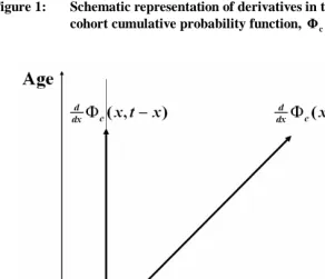
As illustrated here in Figure 1, the labels, “horizontal,” “diagonal,” and “vertical,” refer to directions of change in a Lexis diagram, drawn such that the abscissa and ordinate of the Cartesian plane correspond to the time and age of death, respectively (thus, cohort lifetimes are represented by diagonal lines). The horizontal and diagonal derivatives are obtained, respectively, from the earlier equation for the percentile slope and from the definition of Φc(x,τ) in terms of φc(x,τ). The vertical derivative follows from the

fact that the derivative in the diagonal direction equals the sum of the other two derivatives.

Figure 1: Schematic representation of derivatives in three directions of the

cohort cumulative probability function, Φc(x,τ)

The derivative of Φc(x,τ) in the vertical direction is important because it illustrates that the cross-sectional sum of cohort probability distributions does not in general equal one. For example, if sc(x,t−x)>0 for all x, it follows that

(

)

∫

∫

∫

In this example, since cohort percentile slopes at time t are positive, the timing of death is being delayed or postponed for each successive cohort. This equation illustrates the phenomenon of partial quantum, which occurs whenever the age distribution of events (deaths) is shifting upward over time. Conversely, if the distribution of deaths is shifting uniformly toward younger ages (thus, the timing of death is being advanced or accelerated), then sc(x,t−x) would be negative for all x at time t, and the above sum would be greater than unity (i.e., surplus quantum). Let us refer to φc(x,t−x) as a cross-sectional cohort probability density function.

Assuming that sc(x,t−x)>−1 for all x at time t,

5

it is possible to define the following probability density function:

(

)

φ , (16)

where ) , ( 1 ) , ( ) , ( x t x s x t x s x t x r c c c − + − =

− , and thus 1+sc(x,t−x)=

(

)

function sums to one over the full age range (see equation 15 above), since )

, ( ) ,

(xt x xt x

sc − φc − replaces the missing quantum at age x, assuming sc(x,t−x)>0. 6

Thus, )φ*(x,t is an adjusted cross-sectional cohort probability density function.

5 _{It is theoretically possible for cohort percentiles to have slopes that are less than –1, and their reality has been confirmed by empirical}

observation. For expediency, this situation will be not covered in this paper, as we assume that sc(x,t−x)>−1. Although the formulas of this section remain correct even when cohort percentile slopes dip below –1, the interpretation of the quantities, _φ*(_x,_t) _and µ*_{(x,t), as adjusted}

density functions and adjusted death rates is no longer valid.

6 _{In this discussion we will generally consider the example of cohort percentiles that increase over time, reflecting an increase in longevity. It}

One important feature of the adjusted function, φ*(x,t), is its relationship to the cross-sectional cohort cumulative probability and survival functions, Φc(x,t−x) and

) , (xt x

c −

l , respectively. In the following equation, note that the first integral derives from the definition of Φc, whereas the second integral follows from equation 14:

∫

∫

= −

Φ x x

c

c(x,t x) ₀φ (a,t x)da ₀φ*(a,t)da . (17)

Likewise, it follows that:

∫

∫

= − Φ − = −

x x c

c

c(x,t x) 1 (x,t x) φ (a,t x)da φ*(a,t)da

l . (18)

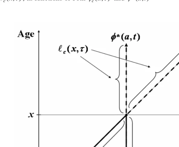
These relationships, linking Φ_c and l_c to φ_c and φ*, are illustrated here in Figure 2A. Following a similar logic, let us define adjusted death rates as follows:

(

)

) , ( 1

) , ( )

, ( ) , ( 1 ) , ( *

x t x r

t x t

x x t x s t

x

c c

− − = −

+

= µ µ

µ . (19)

The cumulative death rate at age x and time t also has two equivalent forms:

∫

∫

=

− x x

c

c xt x at x da at da

H

0

0 ( , ) *( ,)

) ,

( µ µ . (20)

Therefore, the cohort survival probability at age x and time t can be computed using either set of death rates:

{

_∫

} {

_∫

}

=

− x x

c

c(x,t x) exp ₀µ (a,t x)da exp ₀µ*(a,t)da

l . (21)

Figure 2: Illustration of relationship between cumulative quantum for cohorts and “tempo-adjusted” age-specific quantum for periods

A) Cohort cumulative probability of death, Φc(x,τ), and probability of survival, lc(x,τ), as functions of both φc(a,τ) and φ*(a,t)

Note: As discussed in the text, Φc(x,τ)=∫₀xφc(a,τ)da=∫₀xφ*(a,t)da, and ∫

∫∞ = ∞

= Φ − =

x x c

c

c(x,τ) 1 (x,τ) φ(a,τ)da φ*(a,t)da

Figure 2: Continued

B) Cohort probability of survival, lc(x,τ), as functions of both µc(a,τ) and µ*(a,t)

Note: As discussed in the text,

   

 ₋ =    

 ₋

= _∫x _∫x

c

c(x,τ) exp ₀µ(a,τ)da exp ₀µ*(a,t)da

l , where τ=t−x. Compare

4. Alternative measures of period mean lifespan

In addition to life expectancy at birth, e , several other measures of period mean 0

lifespan have recently been put forth (see review by Bongaarts, 2005). Here, we focus on two measures in particular: the “cross-sectional average length of life” (CAL), proposed by Brouard (1986) and Guillot (2003), and “tempo-adjusted” life expectancy at birth, suggested by Bongaarts and Feeney (2002, 2003). In this section, I will explore the mathematical relationship between these and one related measures, plus their connection to period e . 0

In terms of notation, let CAL be denoted *

0

e , and let the Bongaarts-Feeney measure be written as eBF0 . In this section we will also consider a third measure, e0′, or the

mean age at death (MAD) in a constant-birth population. As we shall see, these three period measures are closely related; moreover, they are equivalent in a special case (i.e., when the shift at time t in cross-sectional cohort distributions of age at death is constant across age). However, *

0

e , e0′, and BF

e0 are different in general from the period life

expectancy at birth, e . All four measures are equal only under a very restrictive 0

condition (i.e., that age-specific mortality rates are not changing at time t and have been constant over time for all living cohorts).

A key contention of this article is that *

0

e and e0′ are useful primarily as measures

of population dynamics and, as such, differ fundamentally from e , which is based on 0

the model of a synthetic cohort. As discussed earlier, the synthetic cohort that underlies

0

e is a hypothetical group of people who experience the death rates of the current

period throughout life. In contrast, a model of population dynamics underlies the interpretation of *

0

e and e0′; the key feature of this model is an assumption of a constant

stream of births flowing into the population, arriving at rate of B births per year. If this constant-birth population were subject to the historical mortality conditions of some actual population up until time t, then at that moment its size would be *()

0 t e

B , and the mean age at death observed in the population would be e₀′(t). Although e0(t)

BF

4.1 Relative size of a constant-birth population, e*₀

Both Brouard (1986) and Guillot (2003) have proposed the “cross-sectional average length of life,” a measure known by its acronym, CAL, written here also as *

0

e . By definition,

{

}

exp

) , ( )

( ) ( *

0

0 0

0 0

∫

∫

∫

∫

∞ ∞

∞

= −

=

− =

=

dx t x x dx da t a

dx x t x t

CAL t e

x c

φ µ

l

(22)

where )µ*(x,t and φ*(x,t) are defined as before. Despite the similarity of these formulas to those underlying the calculation of life expectancy at birth, CAL or *

0

e is useful primarily as a measure of population dynamics. As noted by Guillot (2003), in a constant-birth population with a steady inflow of B births per year, the density of survivors at exact age x and time t would be Blc(x,t−x). Therefore, the size of the (hypothetical) constant-birth population that would be observed at time t is a simple function of CAL(t):

) ( * )

, ( )

, ( )

( ₀

0

0 B xt x dx B xt x dx Be t

t

N =

∫

∫

4.2 Mean age at death in a constant-birth population, e0′′′′

, ) , ( ) ( 1 ) , ( ) , ( ) , ( ) , ( ) , ( ) ( ) ( 0 0 0 0 0 0 0

∫

∫

∫

∫

∫

∫

φ by definition, and where =

∫

0 ( , ) *( ,)

)

(t r xt x xt dx

rc c φ is

a (weighted) average of rc(x,t−x) for time t.

Equivalence of the various forms of e0′(t) in equation 24 derives from the following fundamental relationship:7

(

)

) , (

0

0 c xt−x dx=

∫

∫

In other words, rc(t) measures the missing (or surplus) quantum at time t whenever the timing of cross-sectional cohort mortality is being delayed (or accelerated) at that moment. Note that rc(t) also equals the pace of change over time in CAL(t):

. ) ( ) , ( * ) , ( ) , ( * ) , ( 1 ) , ( ) , ( ) ( 0 0 0 t r dx t x x t x r dx t x x t x s x t x s dx x t x t CAL c c c c c dt d dt d = − = − + − = − =

∫

∫

∫

7 _{Some authors have referred to the quantity in equation 25, 1 r(t)}

c

− , as the “total mortality rate,” by analogy to the total fertility rate (Bongaarts

and Feeney, 2003; Guillot, 2005). However, I have chosen not to use this terminology, because )φc(x,t−x is not a mortality rate by the usual

4.3 Tempo-adjusted life expectancy at birth, BF

e0 or e*0

Bongaarts and Feeney (2002, 2003) define “tempo-adjusted” life expectancy at birth as follows:

{

}

∫

∫

∫

∫

µ by definition. Comparing this formula to the

one for e0′(t) given above (i.e., equation 24), we see that each equation resembles one of the classic formulas for life expectancy at birth. It is also useful to compare µ′( tx, ) and )φ′( tx, , which serve as inputs to the calculation of e0(t)

BF

and e₀′(t); in both cases, a measure of age-specific quantum has been inflated (or deflated) by a factor of

(

)

) ( 1−rc t − .

The close relationship between *

0

e and eBF₀ , can be illustrated by re-writing equation 27 as follows:

. ) , ( * ) ( 1 ) , ( 1 exp ) ( 1 ) , ( exp ) ( 0 0 0 0 0

∫

∫

∫

∫

Similarly, we can see the resemblance between *e₀ and e₀′ by re-writing equation 24 as follows:

∫

∫

0 *( , )

) ( 1 ) , ( 1 ) ( 1 ) , ( )

( x t dx

t r x t x r x dx t r x t x x t e c c c c φ φ

In both of the above formulas, the ratio of 1−rc(x,t−x) to 1−rc(t) will be close

to one so long as rc(x,t−x) does not vary widely as a function of age at time t. Bongaarts and Feeney (2002, 2003) assume that rc(x,t−x) is indeed constant with age (their “proportionality” assumption). Since reality resembles this assumption in some cases, the three measures are sometimes approximately equal. However, Guillot (2003) notes that observed differences between CAL and e0′ can be substantial: for French

males the difference was 2.51 years in 2001 and was even larger in earlier decades (e.g., 9.24 years in 1954).

According to Bongaarts and Feeney (2002, 2003), these two quantities, µ′( tx, ) and )φ′( tx, , are “tempo-adjusted” mortality functions. However, unlike µ*(x,t) and

) , ( *xt

φ , )µ′( tx, and φ′( tx, ) are not in general associated with the same probability of survival to age x. That is,

(

)

∫

∫

∫

∫

∫

where +

∫

− − = x c c c da x t x t a a t a r t x r ) , ( ) , ( * ) , ( ) , ( l φ

by definition. In contrast,

{

}

) ( 1 0

0 _{1 ( )} ( , )

) , ( exp ) , (

exp = − −

      − − = ′

−

_∫

_∫

p x c x c t x da t r t a da t

a µ l

µ . (31)

Thus, these two quantities are not the same in general, and for this reason e0(t)

BF

and )

(

0t

e′ are not equal except under special circumstances: when sc(x,t−x) and )

, (xt x

rc − are constant as a function of age x (for a given time t).

Furthermore, as noted also by Feeney (2004, 2005), the general form of tempo-adjusted mortality should involve an appropriate adjustment at each age, not an average correction applied uniformly across the age range. Although Feeney’s notation was different, he also proposed an age-specific adjustment factor of

(

)

) , ( 1 ) , (

1+sc xt−x = −rc xt−x − . As noted earlier in the definitions of µ*(x,t) and

) , ( *xt

mortality functions reflects the shift in the cohort distribution of age at death occurring at that exact age and time, rather than some average value across all ages at time t. For comparison, note the factor of

(

)

As shown earlier, *

0

e (or CAL) can be computed from either µ*(x,t) or φ*(x,t). Thus, CAL is exactly equal to the generalized form of tempo-adjusted life expectancy at birth proposed by Feeney (2004, 2005). In the equations for *

0

e , the factor of )

, (

1+sc xt−x , or

(

)

) , (

1−r_c xt−x − , replaces the lost quantum at age x that results from delay in the timing of mortality from cohort to cohort. The substantive value of this particular interpretation of CAL is dubious (see later discussion). Nevertheless, if this concept is useful at all, then it is worth noting that the generalized form of tempo-adjusted life expectancy at birth equals *

0

e , or CAL, which is different from the original measure proposed under the same label by Bongaarts and Feeney. In fact, _eBF

0 differs

in general from both e*₀ and e0′. As noted earlier, the latter two measures provide

interesting descriptions of population dynamics (in a constant-birth population). Except in the special case when it equals these other two measures, eBF₀ seems to have no substantively interesting interpretation on its own.

4.4 Comparison to period life expectancy at birth, e 0

Even in the special case where *

0

e , e0′, and BF

e₀ are equivalent, their value is typically different from the period life expectancy at birth, e . The latter measure would equal 0

the other three only if the age pattern of mortality were constant over time. However, in the case of a sustained mortality decline, e tends to be higher than the other measures. 0

Let us consider why this difference occurs, focusing in particular on a comparison between e and 0 e*0.

Because )e0(t and e*0(t) equal the sum of period and cohort survival probabilities

across the age range at time t (see equations 1 and 22), it is useful to understand the relationship between lp( tx, ) and lc(x,t−x). As noted earlier, the period survival

single diagonal lifeline of the Lexis diagram. However, such diagonals pertain to different time periods even for a single cohort, and to a wide interval of age and time when we consider the collection of cohorts alive at time t. Thus, an important difference between e0(t) and e*0(t) is that the former is a function of death rates for

time t alone, whereas the latter depends on all death rates (past and present) experienced by cohorts alive at time t.

Furthermore, it is possible to show that

{

}

t x x

t

x x a_dtd

p

c( , − ) = l ( , )exp

∫ ∫

l . (32)

In this equation, the argument to the exponential function is merely the total change in death rates occurring within the triangle of the Lexis diagram that lies below the diagonal lifeline of the cohort born at time t−x, and to the left of a vertical line at time t. Thus, in a situation of sustained mortality decline, the survival probability for a cohort, )lc(x,t−x , would be higher than its corresponding period value, lp( tx, ), by a

factor that depends on the total reduction in mortality risks over this triangular interval of age and time. This representation leads to a useful interpretation of observed differences between e and *0 e0.

As noted already, in a situation of sustained mortality decline, e*₀(t) tends to be lower than e0(t), because lc(x,t−x) tends to be lower than lp( tx, ) across age, x, for

a fixed time, t. Using equation 32, it is possible to convert lp( tx, ) into lc(x,t−x)

simply by factoring out the gains in period survival probabilities due to historical reductions in mortality rates. Likewise, e*₀(t) is lower than e0(t) in this situation because it also does not take into account these past improvements in mortality. This analysis illustrates why the concept of “tempo-adjusted” life expectancy has little value. For a measure of tempo such as e , an adjustment designed to remove the impact of 0

“tempo change” also has the effect of erasing some of the gains in longevity implied by historical reductions in age-specific death rates. For this reason, both *e0 and e0′ are

5. Trends in life expectancy at birth by period and cohort

5.1 Speed of change in historical trends

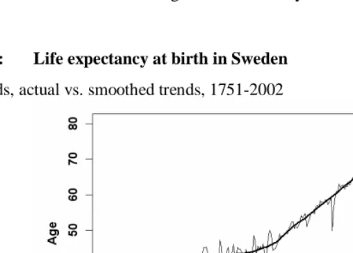
Figures 3A and 3B show actual and smoothed trends in period and cohort life expectancy at birth, plotted in the usual way (by year of death for period e , and year of 0

birth for cohort e ). Then, for comparison with period 0 e , Figure 3C shows the 0

smoothed trend in Swedish cohort e plotted in two ways: by year of birth, and in 0

relation to the time when the cohort’s mean age at death actually occurs.8 Note that the slope of the cohort trend tends to be greater than the slope of the period trend when cohort e is plotted as a function of year of birth, but less when plotted according to the 0

period in which the cohort mean age at death actually occurs.

Figure 3: Life expectancy at birth in Sweden

A) Periods, actual vs. smoothed trends, 1751-2002

Note: The observed trend was smoothed using the LOWESS method (Chambers et al., 1983). Source: Human Mortality Database (2004).

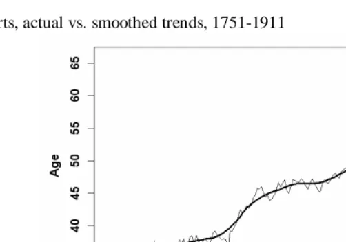
Figure 3: Continued

B) Cohorts, actual vs. smoothed trends, 1751-1911

Notes: (1) See note for Figure 3A. (2) Data employed here for cohorts born after approx. 1890 are incomplete. Therefore, estimates of life expectancy at birth for these cohorts rely on recent period data at very high ages (i.e., above age 90).

Source: Human Mortality Database (2004).

C) Periods vs. cohorts, smoothed trends only

In part, such differences are due to fluctuations over time in historical mortality trends, which affect the mean lifespan of periods and cohorts in complicated ways. Such factors are beyond the scope of the present work. However, in addition to the arbitrary influences of history, there exists an intrinsic difference between period and cohort trends in e due to the fundamental mathematical relationship linking the age 0

and time of death to a decedent’s time of birth.

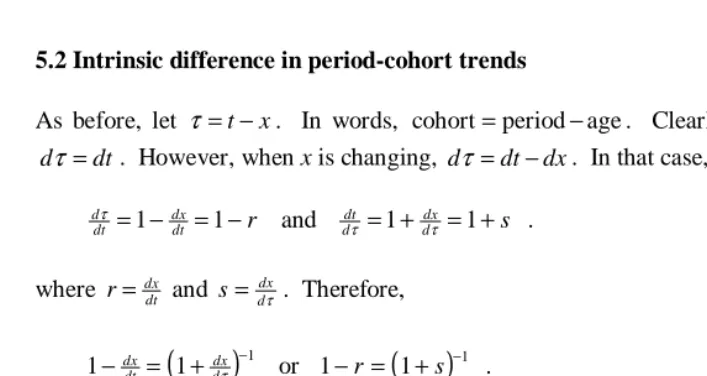
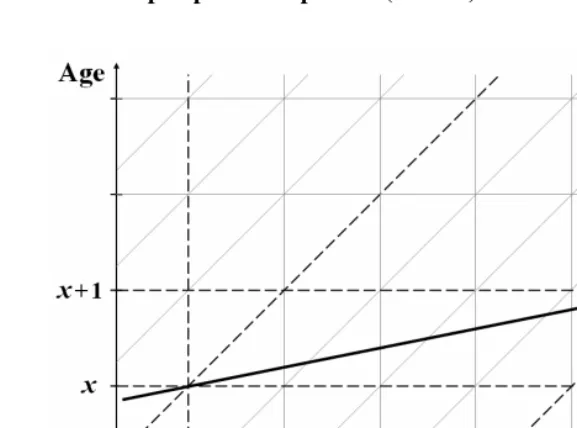
5.2 Intrinsic difference in period-cohort trends

As before, let τ =t−x. In words, cohort=period−age. Clearly, when x is fixed,

dt

dτ = . However, when x is changing, dτ=dt−dx. In that case,

r dt dx dt

dτ =₁− =₁− _{and s} d dx d

dt =₁+ =₁+

τ

τ . (33)

where _r= dx_{dt and}

τ

d dx

s= . Therefore,

(

)

1 1− = +_ddx_τ −

dt

dx _or

(

)

1

1−r= +s− . (34)

It also follows that

s s r

+ =

1 and r r s

− =

1 . (35)

Thus, r and s represent two different measures of the speed of change over time in some function of age. The former is a slope with respect to the timing of the event itself, whereas the latter is with respect to the timing of birth for the cohort that experiences the event. This relationship is valid for any life course event (not only death) and was noted previously by Zeng and Land (2002) in the case of fertility.

Figure 4: Simple example illustrating intrinsic difference in slope of age trend from perspective of periods (r====0.2) and cohorts (s====0.25)

5.3 Period-cohort trends in the linear shift model

In order to elucidate the relationship between period and cohort mortality, it is useful to simulate historical trends using a model of a shifting distribution of age at death. The shift model explored here has three important characteristics:

a) It is linear (i.e., the trend in each percentile of the distribution is linear over time);

b) It is sustained over a long duration (i.e., the shift extends relatively far into both the past and the future); and

c) It is defined in relation to a baseline mortality distribution associated with time

0 = t .9

9 _{Time t=0 is chosen as the baseline for the model in order to keep the formulas as simple as possible. If one wishes to use some other year,}

To simplify the exposition, the linear shift model described here is specified in terms of period mortality at time t=0. It is also possible to define such a model as a function of cohort mortality at time t=0 (i.e., based on a cross-section of cohort mortality distributions at this moment). However, as shown in the Appendix (section A-2.2), a sustained linear shift model yields identical results for those periods and cohorts whose lifespans lie fully within the shift whether the model is defined in terms of period or cohort mortality.10 Therefore, I assume here that the time scale of the shift is relatively long (say, 150 years both forward and backward from time t=0).

As was done earlier for cohorts, let us define percentiles of the period distribution of age at death (i.e., for the synthetic cohort associated with period t) as follows:

x t

a~p(π, )= such that π =Φp(x,t)=1−lp(x,t) , (36)

where Φ_p xt =

∫

0 ( , )

) ,

( φ is the distribution (or cumulative probability) function for age at death in period t. Furthermore, assume that the percentile associated with the same value of π equals y at time t=0:

y

a~p(π,0)= such that π =Φp(y,0)=1−lp(y,0) . (37)

The relationship between these two ages, x and y, can be used to specify the form of historical changes in the age distribution of deaths.

For example, the core assumption of the linear shift model is that the values of x associated with a given y form a straight line, whose slope may vary as a function of age:

t y r y

x= + ( ) for −T <t<T , (38)

where r( y) can take on different values as a function of age, y, subject to certain restrictions (see Appendix, section A-2.3); and T is the duration of the shift both forward and backward from t=0. In general, let us assume that T is sufficiently large to ensure that all cohorts alive at t=0 experience the shift for their entire lives.11

10 _{Note that if the model involves an abrupt change of slope in the percentiles of a mortality distribution at some moment close to the present, say}

0 =

t , then there are important differences between these two approaches.

11 _{As a practical matter, we can assume that all cohort lifespans are finite, and thus that some finite interval, from –T to T, can contain the lifespans}

Note that Φp(x,t)=1−lp(x,t)=π is constant for all combinations of x and t along this percentile contour line. Therefore, another way of describing the core assumption of a linear shift model is that

) ( ) ,

(xt y

p =Φ

Φ or lp(x,t)=l(y) , (39)

where y=x−r(y)t. Thus, Φ( y) and l( y) depict the baseline mortality distribution and survival probabilities for the linear shift model. They are identical to the corresponding period mortality functions associated with time t=0 in the model (i.e.,

) ( ) 0 ,

(y y

p =Φ

Φ and lp(y,0)=l(y) ) .

It is shown in the Appendix (section A-2.1) that in a sustained linear shift model, period life expectancy at birth during the shift interval (i.e., for −T <t<T) has the following form:

t r e t

e0p()= 0+ , (40)

where =

∫

0

0 x (x)dx

e φ ; =

∫

0 r(x) (x)dx

r φ ; and (x) (x) _dxd (x)

dx

dΦ =− _l

=

φ . In the

same model, life expectancy at birth for the cohort born in year τ is as follows:

(

)

τ φ

τ e xs x x dx s x s x x dx s

ec = +

∫

∫

0 0

0

0( ) * ( ) *( ) 1 ( ) *( ) , (41)

where =

∫

0

0 *( )

* x x dx

e φ ; =

∫

0 s(x) *(x)dx

s φ ;

) ( 1

) ( ) (

x r

x r x s

−

= ;

) ( 1

) ( ) ( *

x r

x x

− = µ

µ ;

∫

= −

x da a e

x 0 *( )

) (

* µ

l ; and φ*(x)=l*(x)µ*(x). However, note that equation 41 applies only to those cohorts whose observed (finite) lifespan lies fully within the interval of the period-based shift (i.e., within −T<t<T).

Thus, period life expectancy at time t=0 serves as the baseline value for the linear shift model, i.e., e0(0) e0

p ₌

. Let us consider the relationship between this quantity and cohort life expectancy for two particular cohorts:

a) The cohort born at that moment, i.e., τ=0; and

As indicated by equation 41 above, cohort life expectancy is a function of *

0

e , or

CAL, at time t=0. For the cohort born at time τ =0, this equation simplifies to the following:

(

)

_∫

∫

=

0 0 0

0(0) x 1 s(x) *(x)dx e* xs(x) *(x)dx

ec φ φ . (42)

However, case b) is more complicated.

Obviously the cohort whose average age at death occurs at time t=0 must have been born at some earlier date, say τ=−λ, where λ>0. Setting 0(−λ =) λ

c

e in

equation 41 and then solving for λ yields the following formula:

s e dx x s

x s x e

c c

+ = +

+ = =

−

_∫

1 ) 0 ( )

( * 1

) ( 1 )

( 0

0

0 λ λ φ . (43)

Therefore, the mean ages at death for these two cohorts differ by a factor of 1+s. Also, note that if s(x) is close to constant over the age range, then

(

) ( )

c

e would have a similar value to *e0. Thus, as a

rough approximation, CAL(0) equals the cohort mean age at death that is attained at time t=0 by a cohort born CAL(0) years earlier, assuming linear trends over time in cohort percentiles of age at death.

5.4 Empirical application of the linear shift model

For empirical applications of the linear shift model, we redefine the origin of the time axis in each case so that the current year t is treated as time 0 in the above formulas. The formulas given above for 0(0)

c

e and 0(−λ =) λ

c

e in this model provide motivation for two additional measures of mean lifespan based on cross-sectional cohort mortality patterns at time t. In the first case, define

(

)

_∫

∫

=

0 0 0

0*() 1 ( , ) *( , ) *() ( , ) *( , )

* _{t x s xt x xt dx e t xs xt x xt dx}

Comparing this formula to equation 42 above, it follows that e*₀*(t) equals the average age at death (or life expectancy) for the cohort born at time t, assuming linear trends in cross-sectional cohort percentiles of age at death. In other words, if we create a linear shift model using cohort (not period) mortality patterns observed at time t, the resulting estimate of e0(t)

c

equals e*0*(t). In the second case, let

) ( 1

) ( * * )

, ( * ) ( 1

) , ( 1 )

( 0

0 0

t s

t e dx t x t

s x t x s x t e

c c

c

+ = +

− + =

′′

_∫

Like e*0*(t), this quantity is a linear projection of cross-sectional cohort mortality at time t. If historical changes mimic the linear shift model exactly, then

λ λ = − =

′′() 0( )

0t e t

e c

(compare equation 43 above). Furthermore, even when actual conditions differ from assumptions of the this model, e0′′(t) may serve as a useful approximation of cohort life expectancy for the cohort whose average age at death occurs at time

t

In Figure 5, smoothed trends in Swedish period and cohort life expectancy at birth are compared to these two sets of predictions, e*0*(t) and e0′′(t). These results

demonstrate that the predictions of the linear shift model match reality reasonably well. Therefore, it seems to be possible to use this model to form plausible statements about mortality for individual cohorts based on mortality patterns for the collection of cohorts observed in a cross-section at a moment of time. However, the current purpose of these calculations is not to obtain estimates or forecasts of cohort life expectancy, but rather to provide insights into the relationship between period and cohort mortality. Note that each value of e*0*(t) and e0′′(t) in Figure 5 is based on cohort mortality patterns for a

single year. For this reason, the period of unusually rapid mortality change around the middle of the 20th century produces exaggerated trends in both cases (over-estimating the mean lifespan for cohorts born in those years, and under-estimating it for the cohorts whose mean age at death occurs in those years).

Furthermore, note that

(

)

) ( * )

( 2 0 0

1

0 t e t e t

e t