Creation of Text Document Matrices and Visualization
by Self-Organizing Map
Pavel
Stefanovič, Olga Kurasova
Vilnius University, Institute of Mathematics and Informatics Akademijos str. 4, LT-08663, Vilnius, Lithuania e-mail: [email protected], [email protected]
http://dx.doi.org/10.5755/j01.itc.43.1.4299
Abstract. In the paper, text mining and visualization by self-organizing map (SOM) are investigated. At first, textual information must be converted into numerical one. The results of text mining and visualization depend on the conversion. So, the influence of some control factors (the common word list and usage of the stemming algorithm) on text mining results, when a document dictionary is created, is investigated. A self-organizing map is used for text clustering and graphical representation (visualization). A comparative analysis is made where a dataset consists of scientific papers about the optimization, based on Pareto, simplex, and genetic algorithms. Two new measures are also proposed to estimate the SOM quality when the classified data are analyzed: distances between SOM cells, corresponding to data items assigned to the same class, and the distance between centers of SOM cells, corresponding to different classes. The quantization error is measured to estimate the SOM quality, too.
Keywords: self-organizing map; text mining; text document matrix; document dictionary; quantization error; SOM quality measures; common word list.
1. Introduction
For a long time, self-organizing maps were usually used to solve classification and clustering problems of numerical data, i.e., when the objects analyzed are characterized by the features that acquire numerical values [1], [2], [3]. Recently the self-organizing maps have also been frequently used for different types of data: text [4], [5], [6], audio [7], images [8], etc. The paper deals with applications of self-organizing maps to analyze textual information, i.e., text mining.
A lot of textual information surrounds us everywhere, especially in the Internet. The textual information is produced as web codes, text documents, various scientific papers, etc. It is important to find ways of processing it in order to discover important knowledge significant for decision makers [9], [10], [11], [12]. Some problems arise when the textual information needs to be converted into the numerical one, because the results obtained depend on the ways of conversion. Thus, it is necessary to choose the proper control factors of the conversion.
The main goal of the research is to analyze how well a self-organizing map (SOM) can classify and visualize text documents and how the control factors of text document conversion into numerical data
influence SOM results. There is lack of those researches in scientific literatures. Additionally, two measures to evaluate the SOM quality, when the classified data are analyzed, are proposed and investigated in this paper.
The rest of the paper is organized as follows. Section 2 describes a creation of text document matrices, when text documents are converted into numerical data. In Section 3, a short description of a self-organizing map is presented and new measures of the SOM quality are introduced. The results of experimental investigations are presented in Section 4. Section 5 concludes the paper.
2. Creation of text document matrices
dictionary is a list of words from text files excluding the words that do not satisfy the conditions defined by the control factors.
Descriptions of the control factors, when a document dictionary is being created, are as follows:
• Almost in all text documents, there are numbers and alphanumeric characters. There is no need to include them into the document dictionary, because they do not characterize the text document.
• The word length limit is a number indicating the smallest length of words which will be included into the document dictionary. It is not advisable to include short words such as author’s initials, articles ‘a’, ‘an’, ‘the’, or other not informative words into the dictionary.
• The common word list is a list of the words which will not be included into the document dictionary. Often the words such as ‘there’, ‘where’, ‘that’, ‘when’, etc. compose the common word list. All of them are not important for document analysis, so these words just distort the results. However, the common word list can depend on the domain of text documents. For example, if we analyze scientific papers, the words such as ‘describe’, ‘present’, ‘new’, ‘propose’, ‘method’, etc. also do not characterize the papers and it is not purposeful to include the words into the document dictionary. • The stemming algorithm separates the stem from
the word [13]. For example, we have four words ‘accepted’, ‘acceptation’, ‘acceptance’, and ‘acceptably’. The stem of the words is ‘accept’. Only it is included into the document dictionary. All the other words are ignored.
• The word frequency is a number indicating how many times the word has to be repeated in the text so that it could be included into the dictionary. If a small frequency is chosen, rare words that do not characterize the text document will be included into the document dictionary. Otherwise, if a large frequency is chosen, frequent words will be included into the document dictionary, but not all of them characterize the text document.
Thus, the proper values of these control factors should be chosen in order to get a dictionary that characterizes the text documents as exactly as possible.
According to the frequency of the document dictionary words in the text documents, a so-called text document matrix is created:
�
𝑥11 𝑥12 𝑥13 … 𝑥1𝑛
𝑥21 𝑥22 𝑥23 … 𝑥2𝑛
⋮ ⋮ ⋮ ⋱ ⋮
𝑥𝑁1 𝑥𝑁2 𝑥𝑁3 … 𝑥𝑁𝑛
�. (1)
Here 𝑥𝑝𝑙 is the frequency of the 𝑙th word in the 𝑝th text document, 𝑝= 1, … ,𝑁, 𝑙= 1, … ,𝑛. 𝑁 is the number of the analyzed text documents, and 𝑛 is the number of words in the document dictionary.
Therefore, the document matrix is a matrix the elements of which are equal to frequencies of the document dictionary words in the text documents.
A row of matrix (1) is a vector, corresponding to a document. The vectors 𝑋1,𝑋2, … ,𝑋𝑁 can be used for training SOM, 𝑋𝑝= (𝑥𝑝1,𝑥𝑝2, … ,𝑥𝑝𝑛), 𝑝= 1, … ,𝑁. They are presented to SOM as input vectors. A set of the vectors 𝑋1,𝑋2, … ,𝑋𝑁 composes a dataset analyzed. A data item corresponds to a vector, 𝑛 is a dimensionality of the data item.
Over the past decade, many researches dealing with text mining have been conducted. For this reason, various tools have been created to help analyze the text data. We use the Text to Matrix Generator (TMG) toolbox implemented in Matlab [14] to create text document matrices. The toolbox allows us to construct text document matrices from text documents and to perform various data mining tasks: dimensionality reduction, clustering, classification, etc.
3. Self-organizing maps
Although some modifications of self-organizing maps have been made [15], [16], [17], we use here the general Kohonen algorithm [1]. SOM is a set of neurons, connected to one another via a rectangular or hexagonal topology. Each neuron is defined by the place in SOM and by the so-called codebook vectors.
The learning starts from setting the initial values of components of the codebook vectors 𝑀𝑖𝑗. Usually these values are random numbers in the interval (0, 1). The codebook vectors of neurons 𝑀𝑖𝑗, 𝑖= 1, … ,𝑘𝑥, 𝑗= 1, … ,𝑘𝑦, are adapted according to the learning
rule:
𝑀𝑖𝑗(𝑡+ 1) =𝑀𝑖𝑗(𝑡) +ℎ𝑖𝑗𝑤(𝑡)�𝑋𝑝− 𝑀𝑖𝑗(𝑡)�. (2)
Here 𝑘𝑥 is the number of rows, and 𝑘𝑦 is the number of columns in a rectangular topology of SOM; 𝑡 is the order number of the current iteration; ℎ𝑖𝑗𝑤(𝑡) is a neighboring function. The neuron, the codebook vector 𝑀𝑤 of which, is with the minimal Euclidean distance to 𝑋𝑝, is designated as a winner (the so-called best matching unit, BMU). So, 𝑤 is a pair of indices of the neuron-winner for the vector 𝑋𝑝. The learning is repeated until the maximum number of iterations 𝑇 is reached. After SOM learning, the data 𝑋1,𝑋2, … ,𝑋𝑁 or other data are presented to SOM, neurons-winners for each 𝑋𝑝, 𝑝= 1, … ,𝑁, are found. In such a way, the data items are distributed on SOM and some data clusters can be observed.
amounts of data items from different classes, but put into a SOM cell.
With reference to our previous research [20], we use Gaussian neighboring function:
ℎ𝑖𝑗𝑤=𝛼(𝑡)∙exp�−�𝑅𝑤−𝑅𝑖𝑗�
2
2�𝜂𝑖𝑗𝑤(𝑡)�2 �.
(3)
Here 𝛼(𝑡) is a learning rate and it depends on the number of iterations. The parameter 𝜂𝑖𝑗𝑤 is the neighboring rank of 𝑀𝑖𝑗. Two-dimensional vectors 𝑅𝑤 and 𝑅𝑖𝑗 consist of indices of 𝑀𝑤 and 𝑀𝑖𝑗. The indices show a place of the neuron-winner, the codebook vector of which is 𝑀𝑤, for the vector 𝑋𝑝 and that of the neuron, the codebook vector of which is 𝑀𝑖𝑗, in SOM.
There exist various expressions of the learning rate. One of them is an inverse-of-time:
𝛼(𝑡) =�1−𝑇𝑡� (4)
where 𝑇 is the number of iterations and 𝑡 is the order number of the current iteration.
After training SOM, its quality must be evaluated. Usually quantization error 𝐸QE is calculated:
𝐸QE=𝑁1�𝑁𝑝=1�𝑋𝑝− 𝑀𝑤(𝑝)�. (5)
It shows how well the codebook vectors of neurons of the trained SOM adapt to the input vectors 𝑋𝑝, 𝑝= 1, … ,𝑁. Quantization error (5) is the averaged
distance between the vectors 𝑋𝑝 and the codebook vectors 𝑀𝑤(𝑝) of their neurons-winners.
There is a common case where the data, assigned to some classes, are mapped on SOM. Then it is important to estimate whether the classes compose clusters in SOM. The clusters can be seen when observing maps, but it is important to have quantitative measures. We propose here two new measures. These measures can be applied to SOM, used only for the classified data. When we analyze the classified data, it is important to find how well the data items of different classes separate from one another and how close the same class items are. The first measure 𝐸𝑐 proposed is calculated by formula:
𝐸𝑐 =𝑁1𝑐� � ��𝑍𝑖𝑐− 𝑍𝑗𝑐�𝑘𝑖𝑐𝑘𝑗𝑐+𝑏� 𝑛𝑐
𝑗=1 𝑛𝑐−1
𝑖=1
.(6)
Here 𝑐 is a class label, 𝑐= 1, 2, … ,𝑚, 𝑚 is the number of classes; 𝑁𝑐 is the number of data items from the 𝑐th class; 𝑛𝑐 is the total number of neurons corresponding to the data from the 𝑐th class; 𝑍𝑐= �𝑍1𝑐,𝑍2𝑐, … ,𝑍𝑛𝑐𝑐� is a vector, consisting of indices of the SOM cells, corresponding to the data from the 𝑐th class; 𝑘𝑖𝑐 is the number of the data items from the 𝑐th class in the SOM cell, the indices of which are 𝑍𝑖𝑐; 𝑏 is a penalty, calculated by formula:
𝑏
=
𝑙𝑖𝑐′𝑘𝑖
+
𝑙𝑗𝑐′
𝑘𝑗. (7)
Here 𝑘𝑖 is the number of the data items in the SOM cell, the indices of which are 𝑍𝑖𝑐; 𝑙𝑖𝑐′ is the numbers of data items from other classes than the 𝑐th class in the SOM cell, the indices of which are 𝑍𝑖𝑐.
Therefore, when calculating the measure 𝐸𝑐 (6), the Euclidean distances between indices of all the SOM cells, corresponding to the data from the same class, are computed. If there is more than one data item from the same class in the same SOM cell, the distances are multiplied by the number of data items from the same class in the SOM cells. If there are data items from another class in the same cell, we add a penalty, the size of which depends on the proportion of the number of data from other classes than the class estimated and the number of all data items in the cell.
Measure (6) should be calculated for each class and it shows how the data assigned to the same class are clustered by SOM. The smaller value of the measure means that the data from the same class are clustered better.
The second measure 𝐸center proposed is a distance between the centers of indices of SOM cells, corresponding to data items from each class:
𝐸center=𝑚1� �𝑚𝑑=𝑐+1‖𝑌𝑐− 𝑌𝑑‖ 𝑚−1
𝑐=1 . (8)
Here 𝑚 is the number of classes, 𝑌𝑐 is the center of indices of SOM cells corresponding to the data items from the 𝑐th class, 𝑌𝑐 = 1
𝑛𝑐� 𝑍𝑖
𝑐 𝑛𝑐
𝑖=1 .
The measure determines how far the data, assigned to different classes, are in SOM. The higher value of the measure means that the data from different classes are far from one another.
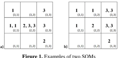
The measures proposed are illustrated by a simple example. Let us have two different SOMs with the same number of cells (Fig. 1). Here the bold number
1, 2, 3 are class labels (𝑐= 1, 2, 3). The pairs of numbers in the corners of the cells are indices of the cells. The indices are used for calculating the values of measures. The values of the measures calculated for SOMs (Fig. 1) are presented in Tables 1–2.
Figure 1. Examples of two SOMs
In Fig. 1a, we see that data assigned to the first class are located in two cells. However, these data are located in three cells in Fig. 1b. Thus, in the first case, the data are clustered more. This fact is confirmed by the first measure (𝐸1= 0.67 for SOM in Fig. 1a, and 𝐸1=1.13 for SOM in Fig. 1b). The value of the first
(𝐸2= 0.71), because not only the data from the second class, but also from the third class are in a cell. So, when we calculate the first measure for the second
class, we add a penalty 𝑏=2
3. Analogous results of the
first measure are obtained for the third class data. In this case, a penalty 𝑏=1
3 is added.
The center indices need to be calculated for the second measure 𝐸center. The center indices of SOM in Fig. 1a are as follows: for the first class 𝑌1=�21
3, 1�,
for the second class 𝑌2= (1.5, 2.5), and for the third
class 𝑌3=�21
4, 2.5�. The center indices of SOM in
Fig. 1b are as follows: for the first class 𝑌1= �223, 113�, for the second class 𝑌2= (1.5, 2.5) and for the third class 𝑌3= (2.5, 3). We can see in Tables 1–2 that the values of the second measure 𝐸center are rather similar. A slightly better result is obtained for SOM in Fig. 1b. In this case, the distance between the centers is large. It means that the data, assigned to different classes, are a little further.
Table 1. Examples of calculation of the measures proposed for SOM in Fig. 1a
Measure Calculation of the measures
First measure for the first class 𝐸1=1
3�2�(1)2+(0)2�= 0.67
First measure for the second class 𝐸2=1
2��(1)2+(1)2+
2
3�= 1.04
First measure for the third class 𝐸3=1
4��(1)2+(0)2+ 2�(1)2+(0)2+
1
3+ 2�(1)2+(1)2+
1
3�= 1.62
Second measure for all classes 𝐸center=1
3���
5
6�
2
+(1.5)2+��1
12�
2
+(1.5)2+��3
4�
2
+(0)2�= 1.32
Table 2. Examples of calculation of the measures proposed for SOM in Fig. 1b
Measure Calculation of the measures
First measure for the first class 𝐸1=1
3��(1)2+(0)2+�(1)2+(0)2+�(1)2+(1)2�= 1.13
First measure for the second class 𝐸2=1
2��(1)2+(1)2�= 0.71
First measure for the third class 𝐸3=1
4�4�(1)2+(0)2�= 1
Second measure for all classes 𝐸center=1 3���1
1 6�
2
+�116�2+��16�2+�123�2+�(1)2+ (0.5)2�= 1.48
4. Experimental investigations
Text mining can be applied in various fields: semantic search engine on the Web, security applications, telecommunications, banks, insurance and financial markets, etc. There are many researches of text mining in the fields. Nowadays, huge amounts of scientific papers have been saved in repositories accessible over the Internet. The search engine helps us to find the desired information in the paper. Often there arises a problem to find similarities of some papers. One way is to explore similar papers according to their title and key words. Another way is to group the papers using clustering methods. The similar papers should fall into one cluster. In this investigation, SOM is applied to cluster and visualize the scientific papers.
As mentioned before, the control factors influence the creation of document dictionaries and text document matrices as well as the results of SOM. If
scientific papers of some different areas are selected for the analysis, they compose not overlapping clusters, and the clusters can be clearly seen in SOM.
The SOM system proposed in [19] is used in experimental investigations. Its exceptional characteristic is an original way of visualizing SOM cells, if the data from different classes are put into a cell. The pie diagrams show the ratio between these data. Let the training set comprises 80 % of all the data, the remaining data being the testing data. We choose SOM of eight rows and eight columns, 𝑘𝑥 =𝑘𝑦= 8.
common word list obtained by TMG is used. The text document matrix has 60 rows and 2368 columns (𝑁= 60, 𝑛= 2368). We see in Fig. 2 that some clusters are observed. Most data items from the same classes form clusters, only some data items are separated from their class clusters. All data from the fourth class (SOM) form one cluster. All data from the third class (optimization) form another cluster. Some data items from the first classes are mixed among the cluster of the second class, because, really, many words can be the same in the papers about artificial neural networks and bioinformatics.
In order to find tendencies how the control factors affect the results, we choose the scientific papers from rather close areas: the papers about optimization based on Pareto, simplexes, and genetic algorithms. The papers were also chosen from full-text scientific databases. The dataset selected consists of 45 papers (15 papers from each field) (𝑁= 45). So, we have 45 vectors 𝑋1,𝑋2, … ,𝑋45 . The vectors 𝑋1,𝑋2, … ,𝑋15 belong to the first class (the papers about simplex), 𝑋16,𝑋17, … ,𝑋30 belong to the second class (the papers
about genetic), and 𝑋31,𝑋32, … ,𝑋45 belong to the third class (the papers about Pareto). The dimensionality 𝑛 of the vectors depends on the number of words in the document dictionary.
Figure 2. SOM of the data, corresponding to the scientific papers about ANN, bioinformatics, optimization, and SOM
Then the papers were converted to text documents, and a document dictionary is created. It can be done in two ways: 1) a researcher manually refers to the words that must be included into the document dictionary;
2) the document dictionary is created automatically from the text documents analyzed.
The text document matrix (1) should be formed according to the document dictionary created. The matrix consists of the frequency of the words, which are in the dictionary.
4.1. Manual dictionary creation I
At first, we create the text document matrix for the dataset that corresponds to the optimization papers, when only three words – ‘simplex’, ‘genetic’, and ‘Pareto’ – are included into the dictionary. In this case, the text document matrix has 45 rows and only
3 columns (𝑁= 45, 𝑛= 3).
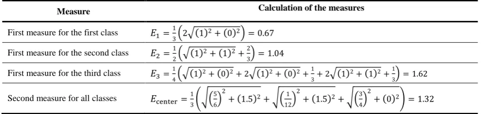
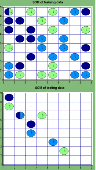
Figure 3. SOM of the data, corresponding to the scientific papers about optimization (manual dictionary creation I)
As we see in Fig. 3, SOM separates all different classes from one another. On the left side of the map for training data, there are data items that correspond to the papers about the simplex algorithm (the first class). The data, corresponding to the papers about genetic algorithms (the second class), are located at the bottom of the map and the data items, corresponding to the papers about Pareto (the third class), are located at the center and the right top corner of the map.
remind that smaller values of the measures proposed 𝐸1, 𝐸2 and 𝐸3 correspond to better SOM results, i.e.,
the clusters on SOM correspond to the data classes. The higher the values of the measure 𝐸center mean, the better the SOM results are, i.e., the class clusters are more separated from one another.
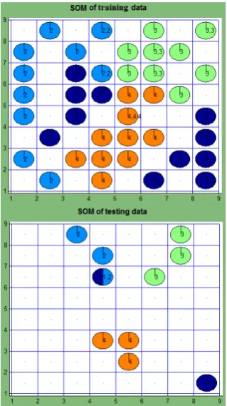
Figure 4. SOM of the data, corresponding to the scientific papers about optimization (manual dictionary creation II)
4.2. Manual dictionary creation II
We can add some other words characterizing the scientific papers into the dictionary. The dictionary consists of the following words: ‘simplex’, ‘programming’, ‘convex’, ‘corner’, ‘vertices’, ‘genetic’, ‘mutation’, ‘crossover’, ‘chromosome’, ‘fitness’, ‘Pareto’, ‘multiobjective’, ‘front’, ‘dominate’, ‘decision’.
SOM is presented in Fig. 4. We also see clusters that correspond to the classes. Only the cluster, corresponding to the first class, splits into two subclusters. Probably, not all the first five words in the dictionary characterize the paper about simplex. It is impossible to compare the SOM results by the quantization error 𝐸QE, because the dimensionality 𝑛 of data items differs. The higher 𝑛, the higher 𝐸QE is. Some values of the measures proposed are worse, some are better comparing to the previous result (see Tables 3–4, No. 1–2). The value of the first measure for the first class 𝐸1 of the training data and that for all the classes 𝐸1, 𝐸2 and 𝐸3 of the testing data are larger. The value of the second measure 𝐸center of the training data is still almost the same, but it is smaller of the testing data. We can draw a conclusion that the
results do not change essentially. Consequently, both dictionaries are acceptable.
4.3. Automatic dictionary creation
As mentioned before, there is a way to create a document dictionary automatically, i.e., the text document is analyzed and specific information is included into the dictionary. In this case, the number 𝑛 of columns in the text document matrix (1) is equal to the number of words in the dictionary. Thus, the number 𝑛 of columns varies depending on the way of the document dictionary creation.
In order to estimate how the control factors of creating a dictionary (usage of the common word list and the stemming algorithm) influence the clustering and visualization results, we have carried out some experimental investigations. Three control factors are fixed and are not changed in all the experiments: numbers and alphanumeric characters are not included into the document dictionary, and the word length limit as well as the word frequency are equal to 3.
4.3.1. Usage of the common word list
The common words that do not characterize the papers analyzed should be included into the common word list. These words are not included into the document dictionary. It is important to select words when composing the list. The task is not trivial, because it depends on the domain of text documents.
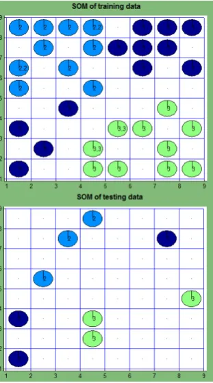
Without the common word list. At first, an experiment is carried out, disregarding the common word list as a document dictionary is being created. In this case, the text document matrix (1) has 45 rows and 3411 column (𝑁= 45, 𝑛= 3441). In Fig. 5, we see that the data compose no clusters, the data classes are intermixed. In all the papers, there are many common words that do not characterize the papers. Thus, it is important to take into account the common word list. Tables 3–4 (No. 3) illustrate that the quantization error 𝐸QE is higher comparing with the error No. 1–2, because the dimensionality 𝑛 of data is higher. The values of the measures proposed are worse (higher 𝐸1, 𝐸2, 𝐸3, smaller 𝐸center) comparing when dictionaries are created manually, except for 𝐸1 for the testing data (see Tables 3–4, No. 3). It means that many inessential words are included into the dictionary when the common word list is not used.
With the common word list obtained by TMG. In the other experiment, the common word list created by the Text to Matrix Generator toolbox [14], is used. This common word list has more than 300 words, such as ‘there’, ‘where’, ‘here’, ‘some’, etc. All of them are ignored in creating the document dictionary as well as the text document matrix.
(No. 3−4), we see that the values of the measures proposed are better comparing with the values, when dictionary is created without the common word list, except for 𝐸2 for the training data. We can draw a conclusion that usage of the common word list is useful.
Figure 5. SOM of the data, corresponding to the scientific papers about optimization (without the common word list)
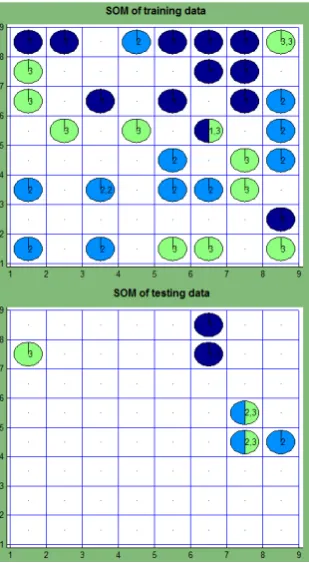
A new common word list. The TMG toolbox has a common word list unsuitable for scientific papers. So, considering that the papers about optimization are analyzed here, we create a new common word list including the words such as ‘function’, ‘fig’, ‘table’, ‘formula’, ‘optimization’, ‘present’, ‘minimum’, ‘maximum’, ‘function’, ‘variable’, etc. The text document matrix has 45 rows and 3157 columns (𝑁= 45, 𝑛= 3157). In this case (Fig. 7), the data from different classes are clustered more than in Fig. 6. In the center of the map, there are data items from the third class. The majority of data from the second class are in the left bottom corner, only one item is in the opposite corner. The majority of data from the first class are located in the left top corner.
The values of the measures proposed are better, except for 𝐸3 for the testing data, comparing the results, when the common word list, obtained by TMG, is used (Tables 3–4, No. 4–5). It means that it is purposeful to compose a common word list taking into account the domain of the scientific papers.
4.3.2. Stemming algorithm
The stemming algorithm separates the stems from the words and only the stems of the words are
included into a document dictionary. In this investigation, the Porter stemming algorithm is used [13]. In Fig. 8–10, the SOM results are presented when the stemming algorithm is used to create a document dictionary. Quantitative evaluations of SOMs are presented in Tables 3–4, No. 6–8. If we compare the SOM results when the stemming algorithm is used and when it is not used, we see that:
• Although the dimensionalities 𝑛 of data are smaller, when the stemming algorithm is used, comparing with the cases without the stemming algorithm, the values of quantization errors 𝐸QE are higher. It means that usage of the stemming algorithm increases the quantization error.
• If any common word list is not used, the usage of the stemming algorithm improves the values of all the measures proposed, except for 𝐸1 for the training data. In the case of testing data, the value 𝐸3 is better when we use common word list and
stemming algorithm, but in other cases 𝐸1,𝐸2,𝐸center are worse.
• If the common word list obtained by TMG is used, the usage of the stemming algorithm improves a half of the SOM results of training and testing data, but other half of results is worse.
• If the new common word list is used, the usage of the stemming algorithm makes worse all the SOM results, except for the case of the training data (𝐸2) and the case of the testing data (𝐸1,𝐸3).
Figure 6. SOM of the data, corresponding to the scientific papers about optimization (with the common word list
Figure 7. SOM of the data, corresponding to the scientific papers about optimization (with a new common word list)
Figure 9. SOM of the data, corresponding to the scientific papers about optimization (with the common word list by
TMG and the stemming algorithm)
Figure 8. SOM of the data, corresponding to the scientific papers about optimization (without the common word list,
but with the stemming algorithm)
Figure 10. SOM of the data, corresponding to the scientific papers about optimization (with the new common word list
and the stemming algorithm)
Thus, it is impossible to draw general conclusions. Sometimes the usage of the stemming algorithm improves the SOM results, but not in all the cases.
Table 3. The values of SOM quality measures for training data
No. Experiment 𝑬𝐐𝐄 𝑬𝟏 𝑬𝟐 𝑬𝟑 𝑬𝐜𝐞𝐧𝐭𝐞𝐫
1 Manual dictionary creation I, 𝑛= 3 2.2624 15.6167 15.4704 17.1277 4.0144 2 Manual dictionary creation II, 𝑛= 15 7.5544 23.3874 12.6742 13.0994 4.0156
3 Without the common word list, 𝑛= 3441 96.1834 24.6728 22.7411 26.0460 1.5694
4 Common word list obtained by TMG, 𝑛= 3198 77.1249 15.7202 25.7068 25.7604 1.6369
5 New common word list, 𝑛= 3157 69.1918 17.8602 21.9739 15.9889 3.4024
6 Without the common word list, but with the
stemming algorithm, 𝑛= 2685 105.7583 25.2302 20.9788 20.4144 2.3180 7 Common word list obtained by TMG and the
stemming algorithm, 𝑛= 2486 88.4657 19.6198 22.3729 26.6322 2.0475 8 New common word list and the stemming
algorithm, 𝑛= 2471 82.7041 19.1223 21.7067 25.3181 2.7453
Table 4. The values of SOM quality measures for testing data
No. Experiment 𝑬𝐐𝐄 𝑬𝟏 𝑬𝟐 𝑬𝟑 𝑬𝐜𝐞𝐧𝐭𝐞𝐫
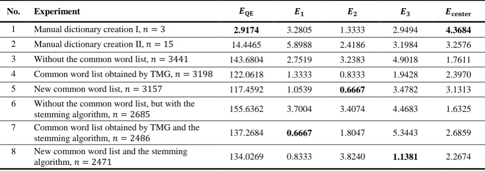
1 Manual dictionary creation I, 𝑛= 3 2.9174 3.2805 1.3333 2.9494 4.3684
2 Manual dictionary creation II, 𝑛= 15 14.4465 5.8988 2.4186 3.1984 3.2576
3 Without the common word list, 𝑛= 3441 143.6804 2.7519 3.2383 4.9018 1.7611
4 Common word list obtained by TMG, 𝑛= 3198 122.0618 1.3333 0.8333 1.9428 2.3970
5 New common word list, 𝑛= 3157 117.4592 1.0539 0.6667 3.4782 3.1313 6 Without the common word list, but with the
stemming algorithm, 𝑛= 2685 155.6362 3.7004 3.4074 4.4683 1.6325 7 Common word list obtained by TMG and the
stemming algorithm, 𝑛= 2486 137.2684 0.6667 1.8047 5.3443 2.6859 8 New common word list and the stemming
algorithm, 𝑛= 2471 134.0269 0.8333 3.8240 1.1381 2.2674
5. Conclusions and future works
In this paper, the influence of control factors (usage of the common word list and the stemming algorithm) for creating document dictionaries on SOM results has been investigated. The scientific papers about optimization, based on the simplex, genetic algorithm and Pareto as the text documents have been used for experimental investigations.
Usually the SOM results are evaluated by the quantization error 𝐸QE, which shows how well the co-debook vectors correspond to the data items analyzed by SOM. However, a problem arises when we want to compare the SOM results in case the dimensionalities 𝑛 of data items differ. Moreover, the quantization error does not show whether the clusters in SOM correspond to the classes of data. Distribution of the data can be observed visually, but it is purposeful to have quantitative measures. So, two measures 𝐸c and 𝐸center have been proposed in this paper, and they as
well as the quantization error 𝐸QE are used to compare the SOM results, varying the control factors. One measure 𝐸c should be computed for each class, and the other one 𝐸center evaluates distances between the
centers of the clusters, corresponding to the classes. Thus, the measures show how well the classified data are arranged in SOM, and whether the clusters obtained correspond to the data classes.
The experiments have shown that the measures proposed are suitable for evaluating SOM when the classified data are mapped onto SOM. A smaller value of the first measure 𝐸c proposed corresponds to SOM, in which the data from a class compose a stronger cluster. The higher value of the second measure 𝐸center corresponds to SOM, in which the clusters of
different classes are farther from one another.
Two types of experiments have been carried out. In the first case, document dictionaries are created manually, i.e., the desirable words are included into a dictionary by researchers. In the second case, document dictionaries are created automatically. The best results for the training data are obtained when the dictionaries are created manually. However, for the testing data, only one value of the second measure 𝐸center is best, in other cases, the results are varying.
When the dictionary is created automatically and any common word list is not used, almost all the values of the measures proposed are worse as compared with that created manually. Usage of the common word list allows us to improve the SOM results. Moreover, it is purposeful to compose the common word list taking into account the domain of the text document analyzed.
If the stemming algorithm is applied in dictionary creation, the stemming improves the SOM results, but not in all cases. In this investigation, the Porter stemming algorithm has been used. In future, it is purposeful to compare the results, obtained by other stemming algorithms.
Another important control factor for creating document dictionaries, word frequency, has not been investigated here. The value of the control factor should be selected carefully, because it greatly influences the results obtained. If a small frequency is chosen, rare words that do not characterize the papers will be included into the document dictionaries, the number of words in the dictionaries will be large, but the data from different classes compose no clusters. If a large frequency is chosen, many frequent words will be included into the document dictionary, but not all of them characterize the paper. But a problem arises due to unequal numbers of all the words in text documents. Usually the length of the scientific papers varies from five to twenty, so the total numbers vary, too. Thus, selection of the word frequency should estimate the ratio between the total number of the words and the word frequency. The evaluation of the influence of the word frequency on the SOM results requires further investigations.
Acknowledgments
This work has been supported by the project ‘Theoretical and engineering aspects of e-service technology development and application in high-performance computing platforms’ (No. VP1-3.1-ŠMM-08-K-01-010) funded by the European Social Fund.
References
[1] T. Kohonen. Self-organizing Maps (3rd ed.), Vol. 30.
Springer-Verlag. 2001.
[2] G. Dzemyda, O. Kurasova, J. Žilinskas.
Multidimensional Data Visualization: Methods and Applications. Series: Springer Optimization and its Applications, Vol. 75. Springer-Verlag. 2013.
[3] J. Pragarauskaitė, G. Dzemyda. Visual decisions in the analysis of customers online shopping behavior.
Nonlinear Analysis: Modeling and Control, 2012, Vol. 17, No. 3, 355–368.
[4] K. Lagus, S. Kaski, T. Kohonen. Mining massive document collections by the WEBSOM method.
Information Sciences, 2004, Vol. 163, No. 1–3, 135−156.
[5] K. Lagus. Text mining with the WEBSOM,
D.Sc.(Tech) Thesis. Helsinki University of Technology, Finland. 2000.
[6] T. Kohonen, H. Xing. Contextually Self-Organized Maps of Chinese Words. In: J. Laaksonen, T. Honkela (Eds.), Advances in Self-Organizing Maps – WSOM 2011, Lecture Notes in Computer Science, Springer-Verlag, 2011, Vol. 6731, 16–29.
[7] R. Mayer. Analysing the Similarity of Album Art with Self-organizing maps. In: J. Laaksonen, T. Honkela (Eds.), Advances in Self-Organizing Maps – WSOM 2011, Lecture Notes in Computer Science, Springer-Verlag, 2011, Vol. 6731, 357–366.
[8] S. Arias, H. Gomezl, F. Prieto, M. Boton, R. Ramos.
Satellite Image Classification by Self-Organized Maps on GRID Computing Infrastructures. In: R. Mayo et al. (Eds.), Proceedings of the Second EELA-2 Conference CIEMAT, 2009.
[9] N. A. Srivastava, M. Sahami. Text Mining Classification, Clustering, and Applications. Chapman & Hall/CRC. 2009.
[10] W. M. Berry, J. Kogan. Text Mining Application and Theory. Wiley, Chichester, UK. 2010.
[11] A. C. Charu, Z. Cheng Xiang (Eds.). Mining Text Data. Springer-Verlag. 2012.
[12] I. Mlýnková, M. Necaský. Heuristic Methods for Inference of XML Schemas: Lessons Learned and Open Issues. Informatica, 2013, Vol. 24, No. 4, 577−602.
[13] M. F.Porter. An algorithm for suffix stripping.
Program: electronic library and information systems, 1980, Vol. 14, 130–137.
[14] D. Zeimpekis, E. Gallopoulos. TMG: A Matlab Toolbox for Generating Term-Document Matrices from Text Collections. Technical Report HPCLAB-SCG 1/01-05, University of Patras, GR-26500, Patras, Greece. 2005.
[15] M. Strickert, B. Hammer. Merge SOM for temporal data. Neurocomputing, 2005, Vol. 64, 39–72.
[16] T. Voegtlin. Recursive self-organizing maps. Neural Networks, 2002, Vol.15, No. 8–9, 979–992.
[17] S. Alonso, M. Sulkava, M. A. Prada, M. Domínguez,
J. Hollmén. EnvSOM: A SOM Algorithm Conditioned on the Environment for Clustering and Visualization. In: J. Laaksonen, T. Honkela (Eds.), Advances in Self-Organizing Maps – WSOM 2011,
Lecture Notes in Computer Science, Springer-Verlag, 2011, Vol. 6731, 61–70.
[18] J. Moehrmann, A. Burkovski, E. Baranovskiy,
G. A. Heinze, A. Rapoport, G. Heidemann. A Discu-ssion on Visual Interactive Data Exploration Using Self-Organizing Maps. In: J. Laaksonen, T. Honkela (Eds.), Advances in Self-Organizing Maps – WSOM 2011, Lecture Notes in Computer Science, Springer-Verlag, 2011, Vol. 6731, pp. 178–187.
[19] P. Stefanovič, O. Kurasova. Visual analysis of self-organizing maps. Nonlinear Analysis: Modeling and Control, 2011, Vol. 16, No. 4, 488–504.
[20] P. Stefanovič, O. Kurasova. Influence of Learning Rates and Neighboring Functions on Self-Organizing Maps. In: J. Laaksonen, T. Honkela (Eds.), Advances in Self-Organizing Maps – WSOM 2011, Lecture Notes in Computer Science, Springer-Verlag, 2011, Vol. 6731, 141–150.