University of New Orleans University of New Orleans
ScholarWorks@UNO
ScholarWorks@UNO
University of New Orleans Theses and
Dissertations Dissertations and Theses
8-10-2005
Adaptive Estimation and Detection Techniques with Applications
Adaptive Estimation and Detection Techniques with Applications
Jifeng Ru
University of New Orleans
Follow this and additional works at: https://scholarworks.uno.edu/td
Recommended Citation Recommended Citation
Ru, Jifeng, "Adaptive Estimation and Detection Techniques with Applications" (2005). University of New Orleans Theses and Dissertations. 311.
https://scholarworks.uno.edu/td/311
ADAPTIVE ESTIMATION AND DETECTION
TECHNIQUES WITH APPLICATIONS
A Dissertation
Submitted to the Graduate Faculty of the University of New Orleans in partial fulfillment of the requirements for the degree of
Doctor of Philosophy in
Engineering and Applied Science
by
Jifeng Ru
B.S., Hefei University of Technology, 1996 M.S., Hefei University of Technology, 1999
Acknowledgment
I would like to express my deepest gratitude to my major advisor, Dr. X. Rong Li, for
his invaluable inspiration, continuous support, and constructive suggestions, which made
it possible for me to complete the Ph.D. dissertation. During my graduate study, I gained
considerable knowledge and insights into problems and techniques in estimation and decision
theory, statistical signal processing and information fusion under Dr. Li’s guidance. All
academic accomplishments I have made during this period are reflection of his efforts and
motivations.
I would also thank Dr. Huimin Chen, Dr. Juliette Ioup, Dr. Vesselin Jilkov, and Dr.
Tumulesh K.S. Solanky for serving on my thesis committee, and for their constructive and
valuable comments on the dissertation. Special thanks go to Dr. Jilkov and Dr. Chen for
their long-term collaboration, fruitful discussions and insightful ideas. Many thanks go to
Dr. Ioup for her suggestions and constant support.
I also want to acknowledge all my friends and members in the Information and Systems
Laboratory, especially Ming Yang, Keshu Zhang, Zhanlue Zhao, Anwer Bash, Peng Zhang,
Ning Li, Lei Lu, Trang Nguyen, Ryan Pitre and Victor Alvarado. With their support
and friendship, I had the great pleasure of carrying out research in such a pleasant working
environment. Furthermore, I would like to thank all the members and staff of the Department
of Electrical Engineering at the University of New Orleans for their support.
This research was supported in part by NSF grant ECS-9734285, NASA/LEQSF grant
(2001-4)-01, ARO grant W911NF-04-1-0274, SBIR N04-241 through Naval Airwarfare
of Energy under Contract DE-AC05-00OR22725 with UT-Battelle, LLC.
Last but not least at all, I want to thank my parents for their unconditional, unending
Contents
1 Introduction 1
1.1 Background . . . 1
1.2 Research Objectives . . . 5
1.3 Thesis Outline . . . 6
2 Hybrid Estimation 9 2.1 Hybrid System . . . 9
2.2 Hybrid Estimation . . . 10
2.3 Multiple Model Estimation . . . 11
2.3.1 Structure of MM Algorithms . . . 12
2.3.2 Development of MM Algorithms . . . 13
2.3.3 Interacting Multiple Model Algorithm . . . 15
2.4 Variable-Structure Multiple Model Method . . . 18
2.4.1 Structure of VSMM . . . 19
3 Variable-Structure MM Estimation with Application in Maneuvering
3.1 Introduction . . . 21
3.2 Expected-Mode Augmentation (EMA) . . . 23
3.2.1 Benefit of Model-Set Augmentation . . . 23
3.2.2 Estimated-Mode Augmentation . . . 25
3.2.3 Expected-Mode Augmentation . . . 25
3.2.4 Practical EMA Algorithms . . . 26
3.3 EMA-IMM Algorithms for Maneuvering Target Tracking . . . 30
3.3.1 Maneuvering Target Tracking . . . 30
3.3.2 Tracking Problem . . . 31
3.3.3 Designs of EMA Algorithms . . . 31
3.4 Performance Evaluation . . . 37
3.4.1 Test Scenarios . . . 37
3.4.2 Simulation Results . . . 38
3.5 Summary . . . 42
4 Adaptive MM approach to Fault Detection, Identification, and Estimation 46 4.1 Introduction and Related Research . . . 46
4.1.1 Conventional Approaches to FDI . . . 47
4.1.2 Multiple Model Approaches for FDI . . . 51
4.1.3 Motivation of VSMM for FDI . . . 52
4.2 Fault Detection Using MM . . . 54
4.2.2 Failure Modeling . . . 55
4.2.3 IMM Estimator for FDI . . . 56
4.3 Hierarchical IMM-FDI . . . 57
4.4 The IM3L Scheme . . . . 59
4.4.1 Benefit of Augmenting Models . . . 60
4.4.2 IM3L Algorithm . . . . 61
4.4.3 IM3L Algorithm for Multiple Failures . . . . 62
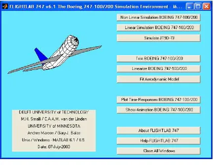
4.5 Boeing 747 Aircraft Simulator . . . 64
4.5.1 Main Functions of the Simulator . . . 64
4.5.2 Linearization of the Boeing 747 model . . . 66
4.5.3 Boeing 747 Aircraft Model . . . 67
4.5.4 VTOL aircraft model . . . 68
4.6 Performance Evaluation . . . 69
4.6.1 Performance Indices . . . 69
4.6.2 GLRT Detector for FDI . . . 71
4.6.3 Simulation Results . . . 72
4.6.4 Discussion . . . 85
4.7 Summary . . . 88
5 Sequential Detection of Change Points 90 5.1 Introduction . . . 90
5.2 Sequential Probability Ratio Test (SPRT) . . . 93
5.4 SSPRT-Based Detector . . . 95
6 Sequential Detection of Target Maneuvers 98 6.1 Introduction and Related Research . . . 98
6.2 Problem Formulation . . . 101
6.3 Existing Algorithms for Maneuver Onset Detection . . . 103
6.3.1 Measurement Residual Based Chi-Square Detector (MR) . . . 103
6.3.2 Input Estimate Based Chi-Square Detector (IE) . . . 104
6.3.3 Input Estimate Based Gaussian Significance Detector (IEG) . . . 105
6.3.4 Generalized Likelihood Ratio (GLR) Detector . . . 106
6.3.5 Marginalized Likelihood Ratio (MLR) Detector . . . 106
6.3.6 CUSUM Based Detector (CUSUM) . . . 107
6.4 Comparison of Existing Detection Algorithms . . . 108
6.4.1 Target Motion Model . . . 108
6.4.2 Four Scenarios . . . 109
6.4.3 Simulation Results . . . 111
6.4.4 Discussions of Existing Maneuver Detection Algorithms . . . 115
6.5 Motivation of Sequential Detection of Target Maneuvers . . . 117
6.6 Sequential Maneuver Detection Algorithm Development . . . 118
6.6.1 Test Statistics of Two Sequential Detection Algorithms . . . 118
6.6.2 Test Statistics of Sequential Detection for a Typical 2D Target . . . . 121
6.7 Performance Evaluation . . . 126
6.7.2 Simulation Results . . . 128
6.8 Summary . . . 132
7 Conclusion and Future Research 134
A Convex Combination of Estimates: EMA approach 137
B MLE of α for Sensor Partial Failures 140
C The PDF of Normal Acceleration 142
D Marginal Likelihood Function under H1 with Gaussian Prior 143
E Marginal Likelihood Function under H1 with Uniform Prior 145
List of Figures
2.1 General structure of MM estimation algorithms . . . 12
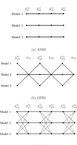
2.2 Filter initializations for AMM, GPB1 and IMM algorithms . . . 16
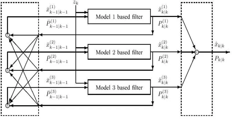
2.3 The structure of the IMM estimation algorithm with three models . . . 17
3.1 Diagraph representation for 13-model set . . . 33
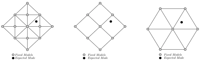
3.2 EMA for 13-, 9- and 7-Model Set Designs . . . 33
3.3 Estimation Errors (DS1 & DS2) . . . 40
3.4 Estimation Errors (Random Scenario) . . . 41
3.5 RMS Position Errors (DS1): 7 + 1 vs. 7 + 2 . . . 44
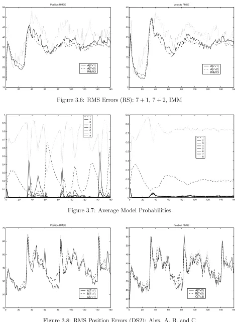
3.6 RMS Errors (RS): 7 + 1, 7 + 2, IMM . . . 45
3.7 Average Model Probabilities . . . 45
3.8 RMS Position Errors (DS2): Algs. A, B, and C . . . 45
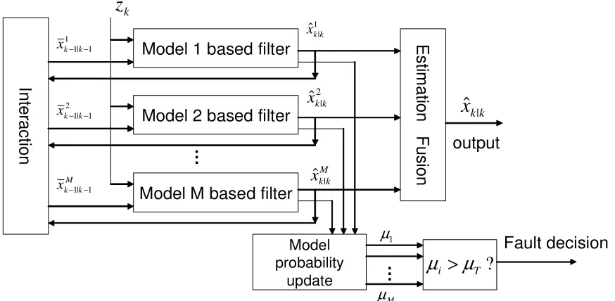
4.1 The block diagram of the IMM algorithm for FDI . . . 57
4.2 A hierarchical structure . . . 58
4.3 Boeing747 simulator . . . 65
4.4 Relationship of FDI performance indices . . . 70
4.6 Case 2 – sequential sensor failures (mild, total failure models) . . . 74
4.7 Case 3 – sequential sensor failures (half failure models) . . . 75
4.8 Case 4 – sequential sensor failures (robustness) . . . 76
4.9 Multiple sensor failures . . . 78
4.10 Case 1 – sequential actuator failures (severe, total failure models) . . . 80
4.11 Case 2 – sequential actuator failures (mild, total failure models) . . . 80
4.12 Case 3 – sequential actuator failures (half failure models) . . . 81
4.13 Case 4 – sequential actuator failures (robustness) . . . 82
4.14 Multiple actuator failures . . . 84
5.1 A change in the mean of a Gaussian process . . . 91
6.1 Onset detection delay for Pfa=5% . . . 112
6.2 Onset detection delay for Pfa=1% . . . 113
6.3 ROC curves for different detectors in SM1 (simple case) . . . 114
6.4 ROC curves for different detectors in SM2 (hard case) . . . 115
6.5 Comparison of CPU time . . . 116
6.6 Asymmetric PDFs of normal acceleration. . . 123
6.7 Gaussian sum approximation of the asymmetric PDF . . . 126
6.8 Posterior probability: normal accelerations change at k= 80 . . . 130
6.9 ROC curves of all detectors for scenario DN . . . 131
6.10 ROC curves of all detectors for scenario DN . . . 131
List of Tables
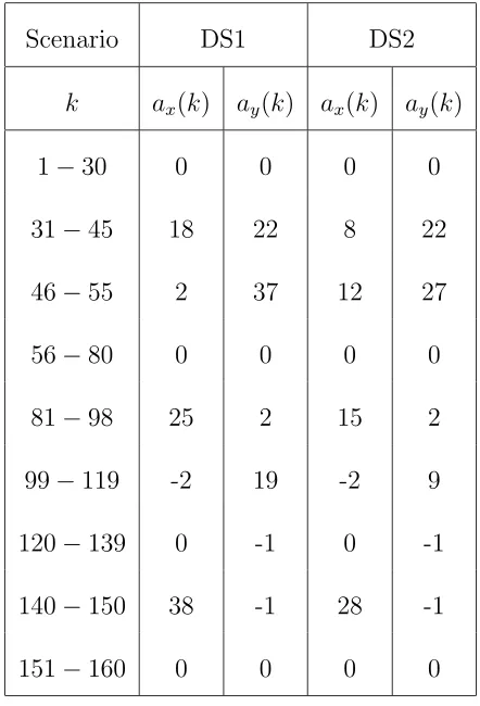
3.1 Deterministic Scenarios’ Parameters . . . 38
3.2 Computational Load . . . 42
4.1 States for linear matrices . . . 66
4.2 Inputs for linear matrices . . . 67
4.3 Detection ranges of HIMM with different model set design for sensor failures 75 4.4 FDI results for sequential sensor failures (VTOL) . . . 77
4.5 FDI results for multiple sensor failures (IM3L, VTOL) . . . . 78
4.6 FDI results for sequential actuator failures (B747) . . . 83
4.7 FDI results for multiple actuator failures (IM3L,B747) . . . . 84
4.8 Computational complexity of different algorithms . . . 85
6.1 Average delay of maneuver onset detection . . . 129
Abstract
Hybrid systems have been identified as one of the main directions in control theory
and attracted increasing attention in recent years due to their huge diversity of engineering
applications. Multiple-model (MM) estimation is the state-of-the-art approach to many
hybrid estimation problems. Existing MM methods with fixed structure usually perform
well for problems that can be handled by a small set of models. However, their performance
is limited when the required number of models to achieve a satisfactory accuracy is large
due to time evolution of the true mode over a large continuous space. In this research,
variable-structure multiple model (VSMM) estimation was investigated, further developed
and evaluated. A fundamental solution for on-line adaptation of model sets was developed
as well as several VSMM algorithms. These algorithms have been successfully applied to
the fields of fault detection and identification as well as target tracking in this thesis. In
particular, an integrated framework to detect, identify and estimate failures is developed
based on the VSMM. It can handle sequential failures and multiple failures by sensors or
actuators.
Fault detection and target maneuver detection can be formulated as change-point
detec-tion problems in statistics. It is of great importance to have the quickest detecdetec-tion of such
mode changes in a hybrid system. Traditional maneuver detectors based on simplistic models
are not optimal and are computationally demanding due to the requirement of batch
pro-cessing. In this presentation, a general sequential testing procedure is proposed for maneuver
detection based on advanced sequential tests. It uses a likelihood marginalization technique
essen-tially utilizes a priori information about the accelerations in typical tracking engagements
and thus allows improved detection performance. The proposed approach is applicable to
Chapter 1
Introduction
1.1
Background
Hybrid systems are complex systems whose states exhibit both continuous and discrete
dynamics. This combination and interaction of the discrete and continuous nature make
this emerging area a particularly challenging field of research. Hybrid systems have been
identified as one of the main directions in control theory and attracted increasing attention
in recent years due to their huge diversity in engineering applications, including system fault
detection, air traffic control, industrial process control, target tracking and communication
networks, etc.
Estimation of the states in a hybrid system subject to structure or parametric uncertainty
is known as hybrid estimation. The conventional solutions to hybrid estimation are
decision-based, where the states are estimated after a decision is made. Specifically, a hypothesis
test is first performed to determine the structure currently in effect and then estimation
estimation has been extensively studied in many areas, and an excellent review of the existing
approaches in the area of target tracking can be found in [50]. Even though the decision-based
approaches have been successfully applied in various applications of hybrid estimation, this
type of solution has clear drawbacks. Since estimation is employed based on a decision, any
possible decision errors on the models are not accounted for in the estimation. Moreover, a
hard decision is taken irrevocably before estimation even though estimation results are often
beneficial to decision making [52].
In recent years, the multiple model approach has become the mainstream approach for
hybrid estimation. In theory, there are certain advantages to use the multiple model
ap-proach. First, for complex systems such as flight control systems, it is often impractical to
represent the whole system using a single model. Second, multiple model representations
provide an easy way to incorporate system information from different sources [91].
The basic idea of the multiple model (MM) estimation is to assume a set of models
describing a hybrid system. It consists of a bank of elemental filters running in parallel, each
based on a particular model representing a possible system behavior or structure, to obtain
conditional estimates; the overall estimate is a certain combination of these
model-conditional estimates; the jumps in the system modes can be modeled as switches/transitions
between the assumed models. Due to these unique features, the MM estimation fits well in
the framework of hybrid estimation and has great success in various fields including target
tracking, air traffic control, fault detection and diagnosis, and communications, etc. [42, 52].
The MM method was initiated in [62] and is now the state-of-the-art approach for many
estimation problems. It has been developed through three generations as identified in [43].
first two generations, the same set of models is used at all times and thus referred to as a
fixed structure-based MM (FSMM) estimation. The third generation allows a variable set of
models adapting to data, leading to a variable structure-based MM (VSMM) estimation.
The existing MM methods with fixed structure usually perform well for problems that
can be handled with a small set of models. Consequently, these methods have a great success
in solving many estimation problems involving structural as well as parametric uncertainty,
particularly in target tracking. However, due to the fact that the true system mode is
often unknown and/or time varying over a large space, an algorithm using a fixed set of a
small number of models cannot yield accurate results. Apart from the dramatic increase in
computation, the research in [43, 48] shows that use of more models in a fixed structure does
not guarantee a performance improvement. To find a way to overcome this dilemma, the
concept and structure of the variable structure MM estimation were introduced in [43, 44,
48, 49, 54], particularly for target tracking, fault detection and identification.
The VSMM is potentially much more advanced than the fixed-structure MM estimation:
besides inheriting the first two generations’ superior processing capabilities, it adapts to the
real environment by augmenting new models or eliminating some existing models according
to applications. This built-in learning mechanism for the model set in the VSMM leads to
an improved performance over the FSMM estimator. The VSMM estimation is especially
powerful for the case when the model set used does not match the possible set of the true
system mode. Due to its open structure and successful applications, the VSMM is gaining
momentum rapidly [42, 43, 44, 55, 59, 86, 87].
typical applications of hybrid estimation due to their common features: both applications
involve continuous-valued parameter estimation such as system states, and discrete
hypothe-ses decision (e.g., possible sensor or actuator failures in FDD, and different target motions
such as constant velocity or constant accelerations in MTT). Thus, it is natural to pose such
problems as one of hybrid estimation.
FDD has been a major issue for modern engineering systems which requires reliability,
availability and security with increasing complexity. In the last two decades, many FDD
techniques have been developed that include hardware redundancy and analytical
redun-dancy based approaches, as surveyed in [9, 23, 26, 29, 99]. However, conventional fault
detection and identification (FDI) algorithms do not deal with failure estimation and state
estimation simultaneously. On the other hand, maneuvering target tracking is a challenging
research topic since target maneuvers are usually unknown. Most of the target tracking
algorithms are hybrid estimation. Therefore, improvement in hybrid estimation, especially
variable-structure based MM estimation, is beneficial to applications of target tracking, fault
detection and identification.
For a hybrid system, since the true system mode jumps due to structure or parametric
change, it is desirable to have a quickest detection, which will provide useful information for
the subsequent state estimation; for example, decision-based approaches for target tracking
or fault tolerant control. Assume that a measurement sequence before and after an unknown
change time has different probability distributions. The objective is to detect the occurrence
of the change as soon as possible under some constraints. This type of problem is usually
formulated as a binary hypothesis testing, known as change point detection in the statistical
According to the sample size, two types of approaches are usually used to detect changes:
fixed-size batch detection including Schewhart’s control chart, geometric moving average,
and cumulative sum control chart; and sequential detection based on sequential probability
ratio test (SPRT) such as Page’s test and Shiryayev SPRT [10, 33, 35, 34]. Due to
un-known maneuver accelerations, target maneuver onset detection can be treated as a typical
application of change point detection.
Many algorithms and techniques have been developed to detect target maneuvers [82],
which can be categorized into two classes: chi-square based and likelihood ratio based tests.
Such detectors are based on simple models and batch processing, and are thus non-optimal
and computationally demanding. Moreover, for tracking applications measurements are
usually available in a sequential manner. As such, it motivates us to investigate the sequential
processing of maneuver detection based on advanced statistical tests. Clearly, this study
could be generalized to other applications under the same formulation such as system fault
detection.
1.2
Research Objectives
The main objective of this research is to formulate problems and develop new algorithms with
regard to hybrid estimation and change point detection for the detection of target
maneu-vers and system faults; more specifically, to develop novel variable-structure algorithms for
multiple model hybrid estimation and apply proposed techniques to target tracking, fault
detection and identification. In essence, a general approach is preferred that adjusts the
small number of models with a desired accuracy level. The proposed approach is expected
to overcome the limitations of the fixed-structure MM estimation and facilitates various
applications of hybrid estimation by providing high cost-effective and robust algorithms.
• The first objective is to present a general variable-structure MM scheme referred to
as expected-mode augmentation (EMA), originally proposed in [49], to enhance the
EMA algorithm with its practical implementation, and to evaluate and analyze its
performance via a generic maneuvering target tracking problem.
• The second objective is to develop an integrated framework to detect, identify, and
estimate failures, including abrupt total, partial and multiple failures, in a dynamic
system. Meanwhile, the proposed approach should provide accurate state estimation
even during failures. This proposed framework based on VSMM is to overcome the
limitations of the existing FDD algorithms.
• The third objective is to investigate the existing target maneuver detection algorithms,
to formulate the problem in a sequential hypothesis setting, and to develop new
sequen-tial detection algorithms based on advanced sequensequen-tial tests to improve the detection
performance, and consequently the tracking performance as well.
1.3
Thesis Outline
This thesis contains seven chapters and five appendices that are organized as below:
Chapter 1 presents the motivation and objectives of this research work.
struc-ture and development of multiple model estimation, in particular, the interacting multiple
model estimator.
Chapter 3 presents a new class of variable-structure algorithms for multiple-model
esti-mation referred to as the expected-mode augmentation (EMA). In the EMA approach, the
original set of fixed models is augmented by a variable set of models intended to match the
expected value of an unknown true mode. These models are generated adaptively in real
time as (globally or locally) probabilistically weighted sums of modal states over the model
set. General formulation, theoretical analysis and justification of the EMA approach are
presented along with three algorithms for its practical implementation. The performances of
the proposed EMA algorithms are evaluated via simulation of a generic maneuvering target
tracking problem.
Chapter 4 proposes two schemes for failure detection, identification and estimation,
in-cluding abrupt total, partial and multiple failures, in a dynamic system. The proposed
algorithms are based on the variable-structure multiple model estimation, which improves
performance due to online adaptation. Using two aircraft examples, the proposed approaches
are evaluated and compared with a widely used single-model residual based generalized
like-lihood ratio (GLR) approach in terms of detection and estimation performance as well as
robustness in the presence of the uncertain noise statistics. Model set design issues are also
discussed along with conclusions and further discussions.
Chapter 5 introduces background information for the change point detection problem
followed by several key sequential detection algorithms.
Chapter 6 addresses target maneuver onset detection based on sequential statistical tests.
developed by using a likelihood marginalization technique to cope with the difficulty of
un-known target maneuver accelerations. The approach essentially utilizes a priori information
about the maneuver accelerations in typical tracking engagements and thus allows improved
detection performance as compared with traditional maneuver detectors. Simulation results
are presented to demonstrate the developed capabilities of the maneuver detectors. The
feasibility of applying proposed sequential algorithms to fault detection is illustrated at the
end.
Chapter 7 draws major conclusions from the research work and provides some further
Chapter 2
Hybrid Estimation
2.1
Hybrid System
A class of simple discrete-time hybrid systems is described by
xk+1 =Fk(sk+1)xk+Gk(sk+1)wk(sk+1) (2.1)
zk+1 =Hk(sk)xk+1+vk(sk) (2.2)
where x is the base state, s is the mode or modal state, z is the measurement, w and v are
independent process and measurement noise. The state in a hybrid system ξ = [x0, s0]0 is
referred to as ahybrid state. Clearly such a system is not linear sincexorz does not depend
on the system state ξin a linear fashion. The system could be deemed as linear if s is given.
For actual systemss could jump at unknown time instants. Jumps between different modes
are used to model abrupt system changes. System (2.1)-(2.2) is known as a Markov jump
linear system if s is a Markov chain
Often s is assumed a homogeneous Markov chain, that is,pij is a constant for all time k.
Base state x is a continuous-valued variable, often referred to as a state variable in a
conventional system, such as position and velocity of a moving object. Mode state s is a
discrete-valued variable for mathematical characterization of a certain behavior pattern or
structure of the system. For example, in the context of fault detection, a normal mode
corresponds to the normal operation of a system. A fault model can be used to represent a
certain failure/degradation in some part of the system. In the context of air traffic control,
the mode of straight and level motion corresponds to the constant velocity motion while
maneuvering modes can be applied to turning or accelerating motions [42]. Different system
modes could be described by different equations with known or unknown parameters.
Such systems (2.1)-(2.2) can be used to model situations whose system behavior
pat-tern undergoes sudden changes, such as system failures and target maneuvers. It provides
a framework particularly suitable for problems with structural as well as parametric
uncer-tainties.
2.2
Hybrid Estimation
In hybrid systems, state estimation subject to structural/parametric uncertainty is called
hybrid estimation in the sense that it combines state estimation and parameter estimation
to deal with simultaneously continuous- and discrete-valued uncertainties. The problem of
hybrid estimation is to estimate the base state and model state based on the sequence of
noisy state measurements along with prior information.
state is estimated after a decision is made. Consequently, the decision errors on models or
possible contributions of estimation to decisions are ignored. Although the limitation is clear
for decision-based approaches, it is still very difficult to come up with effective remedies to
overcome their drawbacks within this framework. Currently, the mainstream approach to
hybrid estimation is the multiple-model (MM) approach, which uses multiple models and
each model represents a possible system behavior or structure. As a result, the multiple
model approach overcomes the difficulty of model uncertainty that conventional
decision-based approaches have to face. The MM approach provides a natural solution for hybrid
estimation.
2.3
Multiple Model Estimation
The basic idea of the multiple model estimation approach is to assume a set of models as
possible candidates of the true mode in the hybrid system. Unique features of MM estimation
include 1) a bank of elemental filters run in parallel to obtain model-conditional estimates;
2) the overall estimate is fused by these model-conditional estimates; 3) transitions between
models are used to model jumps in system mode.
For a Markov jump linear system, the ith model in the MM method is represented by
xk+1 =Fkixk+Gikuk+Tkiwik (2.3)
zk =Hkixk+vki (2.4)
of the system mode are assumed to have the following transition probabilities
πij =P{mjk+1|mik} (2.5)
where mi
k denotes that the ith model is in effect at k.
2.3.1
Structure of MM Algorithms
The operation of MM estimation for hybrid systems is depicted in Fig. 2.1 with only two
models. In general, the application of MM estimation consists of the following steps:
Fusion
Figure 2.1: General structure of MM estimation algorithms
• Model-set design: A major difficulty in the application of MM estimation. It is in
general application dependent and can be done offline or through online adaptation.
Detailed discussions can be found in [52]. The main task in model set design is to select
or construct a set of models possibly covering the system mode space. The performance
of an MM estimator largely depends on the designed model set, especially for problems
• Filter selection: The single-model based filter for each model has to be selected, such as
Kalman filter for a linear problem, an extended Kalman filter for nonlinear estimation,
or a nonlinear filter. Filters based on different models can be of different types. This
step relies on classical estimation theory based on the problem under investigation.
• Cooperation strategy: A main research focus for MM estimation. All possible
coop-erative actions among filters are determined to achieve better performance, such as
pruning of unlikely model sequences, merging of similar model sequences,
individual-ized reconditioning of each filter (e.g., Interacting Multiple Model (IMM) algorithm),
or iterative strategies (like Expectation-Maximization (EM) based algorithms).
• Estimate fusion: This step determines the procedure to combine the individual
model-conditional estimate to yield the overall estimate. It can be achieved either by a
procedure based on a hard decision (i.e., select the estimate from the most likely or at
least not unlikely) or a soft decision (e.g. weighted sum of estimates from every filter).
2.3.2
Development of MM Algorithms
The MM method, state-of-the-art approach for many estimation problems, has been
devel-oped into three generations [52]:
• The first generation, Autonomous MM (AMM) estimation, was initiated in [61, 36, 37]
and widely applied in [65, 66, 67, 72, 96, 22]. In the first generation, each of its
elemental filters operates independently without any interaction with each another. Its
advantage over many non-MM approaches stems from its superior output processing:
to the underlying assumption that the mode does not jump, AMM is not suitable for
problems with frequent changes in system behavior. Instead, it is particularly popular
for problems involving unknown parameters.
• The second generation inherits the first generation’s power of output processing, and its
elemental filters work together as a team via effective internal cooperation. Generalized
Pseudo Bayesian of order n (GPBn) and especially Interacting Multiple-Model (IMM)
are popular algorithms in the second generation. Especially, IMM with its further
development has been successfully applied to a significant number of applications [15,
14, 16, 2, 3, 6, 7, 8]. There exist many cooperation techniques, such as reinitialization
in IMM, iterative iterations for performance enhancement in EM based algorithms,
and other hypothesis reduction strategy.
The model groups in the first two generations have a fixed membership over time and
thus have a fixed structure.
• The third generation allows a variable membership, that is, a variable set of models.
This generation has been known as variable-structure MM (VSMM) method. It is
most suitable in the case where the model set used does not match the set of possible
true modes. The third generation was initiated in [41, 45, 47] and advances have been
further continued in [42, 43, 44, 55, 59, 86, 87, 49, 54, 53].
The first two generations mainly differ in thereinitialization of each elemental filer in the
cooperation strategy. Fig. 2.2 illustrates the difference for three typical algorithms. In the
GPB1 algorithm reinitializes each filter with the previous overall estimate, which carries
information from all filters and thus is the “best possible” common single quasi-sufficient
statistic. In the IMM, each filter has its own reinitialization ¯xi
k−1|k−1 (and ¯Pki−1|k−1), which
forms the best quasi-sufficient statistic of all old information and the knowledge/assumption
that model mi
k matches the system mode at k. The superiority of mixing processing in
the IMM reinitialization has been evidenced by numerous applications [52]. Details of such
algorithms can be found in [6, 7, 8, 52] and references therein.
2.3.3
Interacting Multiple Model Algorithm
The IMM algorithm, originally proposed in [62], has been the main-stream MM algorithm
due to its cost-effective performance and simple scheme demonstrated by a significant number
of successful applications for hybrid estimation. An IMM estimator consists of a bank of
filters, each based on a model matching a particular mode of system; information is utilized
via interaction among filters. The main feature of this algorithm relies on its nature that
different system behavior modes can switch from one to another. This improves its ability to
estimate the state of a dynamic system. The IMM algorithm has three desirable properties:
it is recursive, model conditioned, and has fixed computational load for each cycle [70]. As
aforementioned, compared with other MM algorithms, the superiority of the IMM stems
from the smart individualized reinitialization scheme, which leads to improved performance.
The structure of the IMM estimation algorithm is illustrated in Fig. 2.3 with three
) (
1 | 1
ˆ i
x ()
2 | 2
ˆ i
x ( )
3 | 3
ˆ i
x ()
4 | 4
ˆ i
x
(a) AMM
(b) GPB1
(c) IMM
Figure 2.3: The structure of the IMM estimation algorithm with three models
1. Model-conditional re-initialization: A filter input matching the corresponding mode
is obtained through a mixture of all filter estimates at the previous time, assuming that this
particular mode is in effect at the present time. This step is unique for the IMM estimator
compared with other MM algorithms.
Predicted model probability µi
k|k−1 =
P
mj∈Mk−1
πjiµjk−1
Mixing weight µj|i =π
jiµjk−1/µˆik|k−1
Mixing estimate ¯xi = P
mj∈Mk−1
ˆ
xjk−1|k−1µˆjk|−i1
Mixing covariance ¯Pi = P
mj∈Mk−1
[Pkj−1|k−1+(¯xi
k−1|k−1−xˆ
j
k−1|k−1)(¯xki−1|k−1−xˆ
j
k−1|k−1)
0
]µjk|−i1
2. Model-conditional filtering: This step performs regular filtering including estimation
prediction and update, in a parallel structure for each filter.
Predicted state ˆxi
k|k−1 =Fki−1x¯ik−1|k−1+Gik−1w¯ik−1
Predicted covariance Pi
k|k−1 =Fki−1P¯ki−1|k−1(Fki−1)
0
+Gi
k−1Qik−1(Gik−1)
0
Measurement residual ˜zi
Residual covariance Si
k=HkiPki|k−1(Hki)
0
+Ri k
Filter gainKi
k =Pki|k−1(Hki)
0
(Si
k)−1
Updated state ˆxi
k|k = ˆxik|k−1+Kkiz˜ki
Updated covariancePi
k|k =Pki|k−1−KkiSki(Kki)
0
3. Mode probability update based on the model-conditional likelihood functions. The
model probability plays a key role in the weighting of the state mixing and the fusion.
Model likelihoodLi
k =p[˜zki |mik, zk] =
exp(−(1/2)(˜zi k)
0
(Si k)−1(˜zki))
|2πSi k|
1/2
Model probability µi
k=p[mik |zk] =
µi k|k−1Lik
P
j
µjk|k−1Li k
4. Estimate combination: This yields a total state estimate as the probabilistically
weighted sum of the updated state estimates of all filters.
Overall estimate ˆxk|k=E[xk |zk] = P i
ˆ
xi k|kµik
Overall covariance Pk|k=P i
[Pi
k|k+ (ˆxk|k−xˆik|k)(ˆxk|k−xˆik|k)
0
]µi k
2.4
Variable-Structure Multiple Model Method
The existing MM methods with the fixed structure cannot handel the system well if its true
mode varies over a large space with time or changes frequently. The major reason for the poor
performance of the existing FSMM estimators with a large model set is that many models
in the set are very different from the true system mode in effect at a particular time, thus
the unnecessary “competition” among models degrades the performance [42]. Due to the
nature of the FSMM, it is hard to expect great improvement although further development
is certainly possible, such as the design of a better set of models or the development of better
estimation was initiated in [41, 48] to overcome the fundamental limitations of the fixed
structure MM. The continued research in [42, 43, 44, 55, 59, 86, 87, 49, 54, 53] lays down
the theoretical foundation for hybrid estimation with a variable structure.
The basic idea of the VSMM is to adapt the model set online based on all available
information, in particular, the sequence of the measurements. The real-time measurements
carry valuable information about the system mode being in effect, and thus provide useful
information about the model set.
2.4.1
Structure of VSMM
In VSMM a set of possible models varies with time by online adaptation. In general, each
VSMM algorithm has two tasks:
• Model set adaptation determines at each time the model set to use for the MM
estimation, utilizing posterior information as well as prior knowledge. This is unique
and the most important topic in VSMM estimation. Existing approaches in model
set adaptation can be classified as model-set reduction and model-set augmentation.
It has been shown that combined model-set reduction and augmentation has
signif-icant advantages over model-set switching in terms of tractability, performance, and
generality.
• Model set sequence conditioned estimation intends to provide best possible
es-timates given a model-set sequence, including filter initialization to new models and
cooperation strategies and conditional filtering. The second step is similar to the
Depending on whether the designed total model set can be specified in advance [52],
existing model-set adaptation algorithms for the VSMM can be grouped into two broad
families: active model-sets and model-set generation. In the active model-set family, the
total model set is determined in advance, and a subset is activated adaptively at any given
time. Clearly, the main task for this class of structures is the design of the model subsets,
determination of the candidate subsets, and the decision procedure for switching.
Model-group switching (MGS) is one of the classes with this structure, where the active set is
determined by switching among a number of predetermined subsets of the total model set
[59]. The switching can be done through a soft or hard decision. The likely-model set
(LMS) is another simple class of active model-set structure, where the active set is formed
by deleting the models unlikely to match the true mode at a given time [55]. Another class
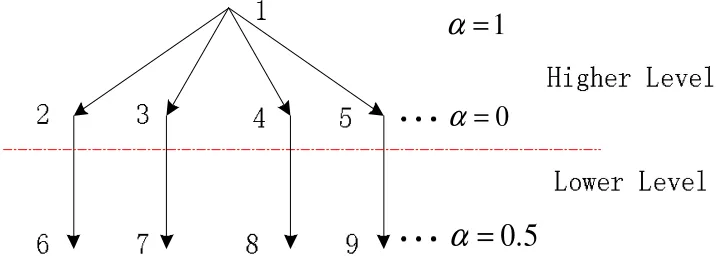
is based on a hierarchical structure, where the active set consists of hierarchical levels of
models [18, 86]. The model subset at a lower level is activated under the guidance of the
higher level.
In the model set generation, new models are generated in real time and thus the model
set cannot be specified in advance. Estimated-mode augmentation is a class for model-set
generation, where the original set is augmented by one or more models that matches an
estimate of the true mode at a given time. The augmented mode can be estimated under
different optimality criteria in principle. Another class is called adaptive grid structure,
where the mode space is quantized unevenly and adaptively based on data as well as prior
information [25, 48, 68]. More details of existing algorithms with adaptive structure can be
Chapter 3
Variable-Structure MM Estimation
with Application in Maneuvering
Target Tracking
3.1
Introduction
In the past, considerable research on multiple model estimation has been undertaken in the
field of hybrid estimation. It is of interest in both military and civilian applications. The
advantage of MM estimation is rooted in the fact that the behavior of a hybrid system cannot
be characterized by a single model for all time, instead a finite number of models may be
adequate to describe the system. Based on the model set, a bank of filters is run in parallel to
obtain model-conditioned estimates, which is used to generate the overall estimates through
certain fusion techniques.
used. Naturally, if the models in the model set are closer to the true mode of the system,
the performance would be better. In many MM applications, the set of possible values of
uncertain system parameters, known as mode space, is continuous. However in reality only
a limited number of models can be used. The common practice is to design a finite set of
models to approximate this mode space. Loosely speaking, the major objective here is to
achieve the best modeling accuracy with a minimum number of models, which is still an open
problem in a general setting, although significant progress has been reported in [45, 58].
To capture various possible unknown mode jumps and in the meantime to have at least
one model close to the true mode, a natural idea is to augment the original model set M
by one or more adaptive models that follow closely the true mode, leading to the so-called
estimated-mode augmentation. Obtaining good candidates for the augmenting models is the
basic idea of estimated-mode augmentation structure. A good candidate for the augmenting
models is the expected value of the true mode since it is statistically closest to the true
mode. This expected mode can be approximated by a sum of modal states weighted by the
corresponding model probabilities, readily available from the underlying MM algorithm. This
expected-mode augmentation (EMA) approach, introduced originally in [49] and furthered
in [54], is systematic and general for all problems with a continuous mode space.
Several researchers have considered similar problems and proposed their solution
tech-niques. For a static MM algorithm, [25] used an initial coarse grid and a subsequent fine
grid while [68] presented a filter bank that moves over a predefined fixed grid according to
a decision logic. It was proposed in [73] to use a moving set of acceleration models
cen-tered around a model whose acceleration is determined by an additional Kalman filter. In
an example of nonstationary noise identification. In [38], an adaptive IMM algorithm for
maneuvering target tracking was proposed that uses an acceleration model determined by
a separate Kalman filter on top of a fixed set of models. Compared with these existing
techniques, not only is the EMA approach much more general and systematic, but it is also
highly cost-effective and easy to implement.
This chapter is organized as follows. In Section 1, the EMA approach is formulated
in a general setting with its theoretical analysis and justification. Three practical baseline
EMA algorithms are proposed in Section 2. Section 3 develops several EMA designs for
maneuvering target tracking. Performance evaluation and comparison of the proposed EMA
algorithms are presented in Section 4 via simulation of a generic maneuvering target tracking
problem. Section 5 provides a conclusion.
3.2
Expected-Mode Augmentation (EMA)
3.2.1
Benefit of Model-Set Augmentation
Denote by s the true mode and by S the mode space (i.e., the set of possible values of
s). Consider the problem of adding a model set C to the original model set M (hence
C∩M =∅). Assume (M ∪C)⊂S. Let
ˆ
xM =E[x|s∈M, z], xˆC =E[x|s∈C, z]
where z stands for measurements. Then according to the total probability theorem, the
estimator of x based on the union of model sets M and C is
ˆ
x=E[x|s∈(M ∪C), z] =µMxˆM +µCxˆC
which is a convex combination of ˆxM and ˆxC. Then, following the derivation in Appendix
A, we have
Lemma If ˆxM and ˆxC are unbiased with uncorrelated estimation errors, which can be
assumed in most cases, use of the union of M and C is better than use of M alone if and
only if
µC <
2mse(ˆxM)
mse(ˆxM) + mse(ˆxC)
where mse(ˆxM) and mse(ˆxc) stand for the mean-square error of ˆxM and ˆxC, respectively.
This inequality is always satisfied if ˆxC is better than ˆxM. Even if ˆxC is worse than
ˆ
xM, ˆx is still better than ˆxM provided µC satisfies the above inequality. If ˆxM and ˆxC have
correlated estimation errors (i.e., E[˜x0
Mx˜C] 6= 0), ˆx is still better than ˆxM if and only if
E[˜x0
Mx˜C]< E[˜x0Mx˜M] = mse(ˆxM), where ˜x=x−xˆ is the estimation error.
Note that this result, which holds when M ∪C ⊂ S, does not contradict the finding
presented in [48] that the optimal use of more models is not necessarily better, because
the above result would not necessarily be correct if C ⊂ S were not true. Since here we
focus on problems with a continuous mode space, M ∪C ⊂ S holds in general and thus
ˆ
xα = (1−α)ˆxM +αxˆC with some α will be better than ˆxM. As a consequence, optimal
use of more models for such problems does improve performance because its estimate ˆx
cannot be worse than ˆxα. Of course, this holds true only under the simplifying assumption
3.2.2
Estimated-Mode Augmentation
In principle, the augmented model can be estimated under any optimality criterion, such as
• expected-mode augmentation: the augmented model is the one based on the condition
mean
ˆ
mM M SEk =E[sk|sk ∈Mk, zk]
whereMk and zk stand for the model set and measurements sequence at timek,
respec-tively.
• maximum-likelihood model augmentation: the augmented model is the one with the
largest likelihood
ˆ
mM Lk = arg max
m f(z
k
|sk=m)
• maximum posterior model augmentation: the augmented model is the one with the
maximum model probability
ˆ
mM APk = arg max
m P(sk =m|z
k)
A promising alternative is to augment the model set also by the predicted modes, such as
ˆ
mM M SE
k+1|k = E[sk+1|sk ∈ M, Mk−1, zk] =
P
mj∈Mmjµ
(j)
k|k, ˆmM Lk+1|k = arg maxmf(zk|sk+1 =m),
ˆ
mM AP
k+1|k = arg maxmP(sk+1 =m|zk), to anticipate the next mode transition, leading to what
can be called predicted-mode augmentation.
3.2.3
Expected-Mode Augmentation
An expected-mode augmentation (EMA) to the VSMM was originally proposed in [49]. Its
[53, 54]. The expected mode is the expected value of the true mode. It is a good model
candidate since it is statistically closest to the true mode. This expected mode (conditional
mean) can be approximated by a sum of modal states weighted by the corresponding model
probabilities, readily available from the underlying MM algorithm
ˆ
mM M SEk =E[sk|sk∈Mk, zk] =
X
mj∈M
mjµjk|k (3.1)
whereµjk|k denotes the updated probabilities of model j being the correct one, andmj is the
parameter value that characterizes model j.
3.2.4
Practical EMA Algorithms
We now describe practical EMA algorithms. For simplicity of presentation, we assume that
the IMM mechanism is used for model-conditioned reinitialization [52].
The proposed EMA algorithms involve the following main functional modules
• EMA Mk :=M+(M1, . . . , Mq): expected mode augmentation procedure;
• VSIMM[Mk, Mk−1]: recursion for variable structure IMM estimation that uses model
sets Mk−1 and Mk at timek−1 and k, respectively;
• EF[M0
k, Mk00;Mk−1]: procedure for estimation fusion of two estimates resulting from
VSIMM[M0
k, Mk−1] and VSIMM[Mk00, Mk−1] recursions, respectively, where Mk0 and Mk00
are discussed later.
The VSIMM and EF functions have been developed, utilized, and documented in several
publications on VSMM estimation [43, 59, 57, 55]. For the EMA procedure, a more detailed
Consider a generic cycle from timek−1 to k. Suppose that the model set Mk−1 used at
k−1 is given. Three basic EMA algorithms are given in Tables 1, 2, and 3, respectively, using
different schemes for determination of the model set M needed to obtain the expected-mode
setEk =E(M;M1, . . . , Mq) at timek. Choices of M1, . . . , Mq are discussed later. The main
difference among the three algorithms lies in how the expected-mode set Ek is determined.
Algorithm A (Step 1) uses Mk−1 (including Ek−1) but not the current measurement zk to
determine Ek. On the contrary, Algorithm B (Step 2) uses zk but not Ek−1 to determine
Ek. Algorithm C (Step 3) uses both zk and Ek−1 to determine Ek. In general, Algorithm
B should outperform Algorithm A at the time instant of a system mode jump (e.g., with a
faster response and hence a smaller peak error) because of the timely information included in
zk, while Algorithm A should have a better steady-state performance due to the more direct
utilization of the old expected modes. Algorithm C provides a trade off between steady-state
performance and fast response.
Algorithm A is the simplest, while Algorithm C is the most sophisticated. Thanks to
the optimal estimation fusion formulas described in [43], the computational complexities of
Algorithms B and C increased by the use of the current measurement zk to determine Ek
are quite limited.
The above algorithms can be integrated to yield more sophisticated algorithms with
improved performance. For example, we can use Ek = EkA ∪EkB as the set of expected
modes, whereEA
k and EkB are the sets of (predicted and updated) expected modes obtained
by Algorithms A (Step 1) and B (Step 2), respectively; or more preferably, we may use
Ek = EkA∪EkC as the set of expected modes, where EkA and EkC are the sets of (predicted
in Step 3, respectively, which is equivalent to replacing Step 5 of Algorithm C by running
EF[M0
k, Ek;Mk−1].
In Step 1 of Algorithm A, use of the predicted model probabilities at the current time
step {µ(ki|)k−1}mi∈Mk−1 amounts to ¯mk = ¯mk|k−1 and should be superior to use of the updated
model probabilities at the previous time step{µ(ki−)1|k−1}mi∈Mk−1, which amounts to assuming
¯
mk= ¯mk−1|k−1. The same is true for Algorithm C. Both sets of model probabilities are readily
available from an MM estimator.
Table 1. One cycle of EMA Algorithm A
S1. Obtain Ek=E(Mk−1;M1, . . . , Mq) using the predicted model probabilities
{µ(ki|)k−1}mi∈Mk−1
S2. ForMk =Ek∪(Mk−1−Ek−1), run VSIMM[Mk, Mk−1] to obtain the overall estimates,
error covariances, and model probabilities nxˆ(ki|)k, Pk(|ik), µ(ki|)ko
mi∈Mk
Table 2. One cycle of EMA Algorithm B
S1. For Mf =Mk−1−Ek−1, run VSIMM[Mf, Mk−1] to obtain
n
ˆ
x(ki|)k, Pk(|ik), µ(ki|)ko
mi∈Mf
S2. Obtain Ek=E(Mf;M1, . . . , Mq) using the current updated model probabilities
{µ(ki|)k}mi∈Mf
S3. Run VSIMM[Ek, Mk−1] to obtain
n
ˆ
x(ki|)k, Pk(|ik), µ(ki|)ko
S4. Run EF[Mf, Ek;Mk−1] to obtain overall estimates, error covariances, and model
prob-abilities nxˆ(ki|)k, Pk(|ik), µ(ki|)ko
mi∈Mk
in the set Mk=Mf ∪Ek
Table 3. One cycle of EMA Algorithm C
S1. Obtain E0
k=E(Mk−1;M1, . . . , Mq) using the predicted model probabilities
{µ(ki|)k−1}mi∈Mk−1
S2. For M0
k=Ek0 ∪(Mk−1−Ek−1), run VSIMM[Mk0, Mk−1]
S3. Obtain Ek=E(Mk0;M1, . . . , Mq) using thecurrent updated model probabilities
{µ(ki|)k}mi∈Mk0
S4. Run VSIMM[Ek, Mk−1]
S5. For Mf = Mk−1 −Ek−1, run EF[Mf, Ek;Mk−1] to obtain overall estimates, error
co-variances, and model probabilities nxˆ(ki|)k, Pk(|ik), µ(ki|)ko
mi∈Mk
3.3
EMA-IMM Algorithms for Maneuvering Target
Tracking
3.3.1
Maneuvering Target Tracking
Tracking is the estimation of the state of a moving target based on measurements. The target
state usually consists of kinematic components (position, velocity, acceleration, etc.) and
other parameters [5]. The target motion uncertainty is one of the major challenges of target
tracking, i.e., a target may undergo a known or unknown maneuver during an unknown time
period. Clearly, this problem involves both the estimation of continuous-valued parameters
such as target states and the detection of target motions. Thus, it is natural to pose target
tracking as a hybrid estimation problem involving both continuous and discrete uncertainties.
In general, a nonmaneuver motion and different maneuvers can be described only in
different motion models. The use of an incorrect model often leads to unacceptable results.
When tracking a maneuvering target, it is thus crucial to determine reliably and timely the
right model to use [43]. Currently the multiple model method is a major approach to target
3.3.2
Tracking Problem
The target motion-measurement model is
xk+1 =F xk+G[a(k) +wk]
zk+1 =Hxk+1+vk+1, k= 0,1,2, . . .
wherex,(x,˙x,y,˙y)0 denotes the target state,a,(ax, ay)0 is the acceleration,wk ∼ N[0, Q]
is the acceleration process noise, z = (zx, zy)0 is the measurement, vk ∼ N [0, R] is the
random measurement error, and F = diag[F2, F2] and G= diag[G2, G2] with
F2 =
1 T 0 1
, G2 =
T2/2
T
, H=
1 0 0 0
0 0 1 0
The unknown true acceleration is assumed piecewise constant, varying over a given
con-tinuous planar region Ac. In the MM framework, we consider a generic finite set (grid) of
acceleration values:
Ar ,{ai ∈Ac :i= 1,2, . . . , r} (3.2)
which defines the total model set. We approximate the evolution of the true acceleration over
the quantized setArvia a Markov chain model, that is,a(k)∈Arwith givenP {a(0) =ai}=
Pi and P{a(k) =aj|a(k−1) =ai}=πij for i, j = 1,2, . . . , r.
3.3.3
Designs of EMA Algorithms
Consider the following well-known example of [1], [46], [60], [73], [41], [57], [55]. The mode
space is defined as
i.e., the maximum acceleration in any coordinate direction is about 4g(g = 9.8m2/s). It
is, however, more appropriate that the target acceleration model be independent of the
orientation of the observer’s coordinate system. That is why we consider
Ac0 ,n(ax, ay) :
q a2
x+a2y ≤40
o
IMM13
The basic 13-model set design A13, obtained after quantization ofAc, is
a1 =ρ[0,0]0 a2 =ρ[1,0]0 a3 =ρ[0,1]0
a4 =ρ[−1,0]0 a5 =ρ[0,−1]0 a6 =ρ[1,1]0
a7 =ρ[−1,1]0 a8 =ρ[−1,−1]0 a9 =ρ[1,−1]0
a10=ρ[2,0]0 a11 =ρ[0,2]0 a12 =ρ[−2,0]0
a13=ρ[0,−2]0
with ρ= 20≈2g.
The transition relations among models are easily understood in terms of the directed
graph (i.e., digraph) representation of an MM, introduced in [41]. The topology of model set
A13 is depicted in Figure 3.1. Each model is viewed as a point in the mode (acceleration)
space. An arrow from one model to another indicates a legitimate model switch (self-loops
are omitted) with nonzero probability. All details can be found in [41], [57]. Note that for
simplicity in A13 a model is allowed to switch to its nearest neighbor(s) only. Better results
could be obtained if other types of model switching are allowed, such as those between second
nearest neighbors (e.g., a2 and a3, and a6 and a10) (see [55]). The values of the transition
Figure 3.1: Diagraph representation for 13-model set
Fixed Models Expected Mode Fixed Models Expected Mode Fixed Models Expected Mode
Figure 3.2: EMA for 13-, 9- and 7-Model Set Designs
EMA{13+1}
As illustrated in Figure 3.2 (a), the expected-mode augmented (EMA) set of the fixed-grid
model A13 is A13+1(k) ,
A13, ˆak|k−1 , where ˆak|k−1 = Paj∈A13+1(k−1)µ
(j)
k|k−1aj and µ
(j)
k|k−1
are the predicted model probabilities available from the IMM estimator. Note that ˆak|k−1, as
a convex combination of the points of A13, covers the entire continuous acceleration region
Ac, i.e. ˆa
k|k−1 can be any point in Ac, depending on µ(kj|)k−1. The values of the transition
P = [pij] of A13as follows:
π1,14= 0.01, πi,14 = 0.05, i= 2, 3, . . . , 13
πjj =pjj −πj,14, π14,j = 0.01, j = 1,2, . . . , 13
and all other elements remain unchanged (i.e., πij =pij).
The implementation of the corresponding IMM estimator with EMA-Algorithm A as
given in Table 1 is straightforward withA13+1(k). This implementation is referred to as the
EMA-A{13+1}.
EMA{9+1}
This model, illustrated in Figure 3.2 (b), is obtained from EMA{13+1} by deleting its
internal nonzero models (vertices) a2, a3, a4, a5.1 Its TPM used in the simulation was
.96 .001 .001 .001 .001 .001 .001 .001 .001 .032
.01 .75 .0 .0 .0 .01 .0 .0 .01 .22
.01 .0 .75 .0 .0 .01 .01 .0 .0 .22
.01 .0 .0 .75 .0 .0 .01 .01 .0 .22
.01 .0 .0 .0 .75 .0 .0 .01 .01 .22
.01 .01 .01 .0 .0 .75 .0 .0 .0 .22
.01 .0 .01 .01 .0 .0 .75 .0 .0 .22
.01 .0 .0 .01 .01 .0 .0 .75 .0 .22
.01 .01 .0 .0 .01 .0 .0 .0 .75 .22
.002 .002 .002 .002 .002 .002 .002 .002 .002 .982
1
The variant with deleting a6, a7, a8, a9 was also examined, but the one presented here showed better
The implementation of the corresponding IMM estimator with EMA-Algorithm A for this
design is referred to as the EMA-A{9+1}.
EMA{7+1} & EMA{7+2}
In order to cover more efficiently the true acceleration setAc
0defined above we also considered
the diamond fixed model set design A7 [45], illustrated in Figure 3.2 (c):
a1 =ρ[0,0]0 a2 =ρ[2,0]0 a3 =ρ1, √
30
a4 =ρ
−1,√30 a5 =ρ[−2,0]0 a6 =ρ
−1,−√30
a7 =ρ
1,−√30
withρ= 20. Two types of EMA designs based onA7were considered—single-model
augmen-tation, denoted by A7+1(k), {A7, ˆa8(k)} (Fig. 3.2) and two-model augmentation, denoted
by A7+2(k), {A7, ˆa8(k),aˆ9(k)}. All Algorithms A, B, and C presented above were
imple-mented for bothA7+1andA7+2. The corresponding algorithms are denoted as EMA-A{7+i},
EMA-B{7+i}, EMA-C{7+i}, i= 1,2, respectively. The EMA{7+1} and EMA{7+2}
algo-rithms always use ˆa8(k) = ¯m1 as computed by (3.1). The EMA{7+2} algorithms also
compute ˆa9(k) as the probabilistically weighted sum of the accelerations of the three most
probable models in the respective model set.
respectively were used in the simulation
.894 .001 .001 .001 .001 .001 .001 0.1
.05 .65 .05 .0 .0 .0 .05 0.2
.05 .05 .65 .05 .0 .0 .0 0.2
.05 .0 .05 .65 .05 .0 .0 0.2
.05 .0 .0 .05 .65 .05 .0 0.2
.05 .0 .0 .0 .05 .65 .05 0.2
.05 .05 .0 .0 .0 .05 .65 0.2
.001 .001 .001 .001 .001 .001 .001 0.993
and
.964 .001 .001 .001 .001 .001 .001 .015 .015
.05 .65 .05 .0 .0 .0 .05 .1 .1
.05 .05 .65 .05 .0 .0 .0 .1 .1
.05 .0 .05 .65 .05 .0 .0 .1 .1
.05 .0 .0 .05 .65 .05 .0 .1 .1
.05 .0 .0 .0 .05 .65 .05 .1 .1
.05 .05 .0 .0 .0 .05 .65 .1 .1
.01 .01 .01 .01 .01 .01 .01 .9 .03
.01 .01 .01 .01 .01 .01 .01 .03 .9
All other parameters of the IMM algorithms implemented in the simulation were the
3.4
Performance Evaluation
3.4.1
Test Scenarios
The performances of all nine MM tracking algorithms (viz., IMM13, EMA-A{13+1},
EMA-A{9+1} and EMA-A{7+i}, EMA-B{7+i}, EMA-C{7+i}, i = 1,2) were investigated first
over a large number of deterministic maneuver scenarios with fixed acceleration sequences.
Deterministic scenarios serve to evaluate algorithms’ peak errors, steady-state errors and
response times. We present two of them, referred to as DS1 and DS2, in the sequel. Their
acceleration values are given in Table 3.1. The other parameters for both scenarios are
T = 1s, Q= 0, R= 1250I, x0 = [8000, 25, 8000, 200]0.
Note that while the acceleration values in DS1 are relatively close to the fixed grid points
of IMM13, in DS2 they are deliberately chosen far apart from the grid points. As such, for
the fixed structure estimator IMM13 the scenario DS2 is more difficult than DS1.
To provide performance comparison as fair as possible performance comparison over
an ensemble of maneuver trajectories, the algorithms were tested on a random scenario,
developed in [57], [55]. With such a scenario, it is difficult, if not virtually impossible, to
design an MM estimator with subtle tricks that are effective only for certain scenarios. In
the random scenario the acceleration vectora(t) =a(t)∠θ(t) is a 2-dimensional semi-Markov
process which undergoes sudden jumps from a state with a magnitude a and phase θ to
another one after staying in it for a random period of time. Briefly, the model assumes: the
sojourn timeτkof the state and varianceσ2; the acceleration magnitudeak+1 has probability
massesP0 andPM to be zero and maximum, respectively, and uniform in between; the angle
Table 3.1: Deterministic Scenarios’ Parameters
Scenario DS1 DS2
k ax(k) ay(k) ax(k) ay(k)
1−30 0 0 0 0
31−45 18 22 8 22
46−55 2 37 12 27
56−80 0 0 0 0
81−98 25 2 15 2
99−119 -2 19 -2 9
120−139 0 -1 0 -1
140−150 38 -1 28 -1
151−160 0 0 0 0
σ2
θ otherwise. All details and discussions were given in [57]. In the simulation we used the
following parameters:
¯
τ = ¯τM + amaxamax−a(¯τ0−τ¯M), στ = 121τ¯a
¯
τM = 10, τ¯0 = 30, PM = 0.1, amax= 37
σθ =π/12, P0 = 0.8, ak=amax
3.4.2
Simulation Results
Two main tasks were of interest in the simulation:
designs (viz., EMA-A{13+1}, EMA-A{9+1} and EMA-A{7+1}) and compare with
the fixed structure algorithm (IMM3).
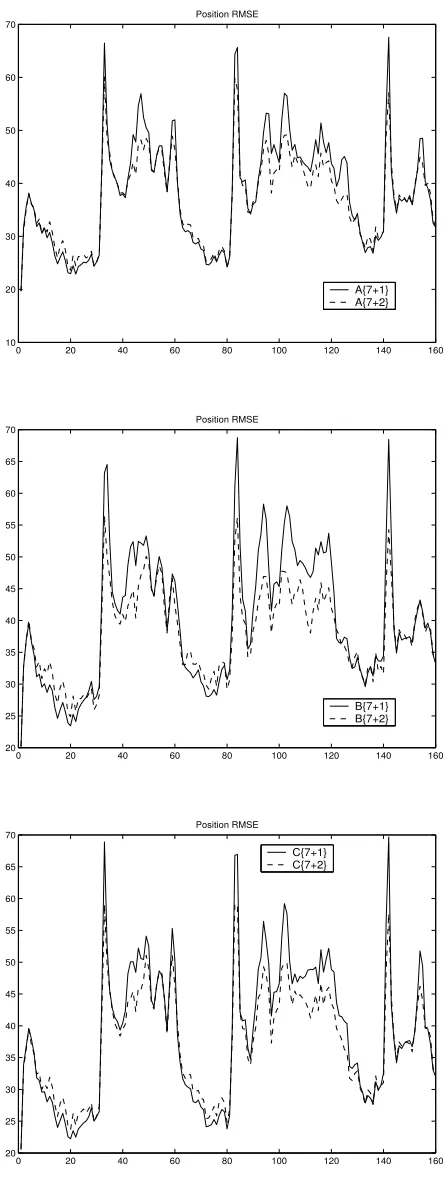
b) Evaluate and compare the performances of the different EMA algorithms (EMA-A,
EMA-B, EMA-C) with different number of models within a particular design (viz.,
A{7+i}).
EMA-A{13+1}, EMA-A{9+1} and EMA-A{7+1} vs. IMM
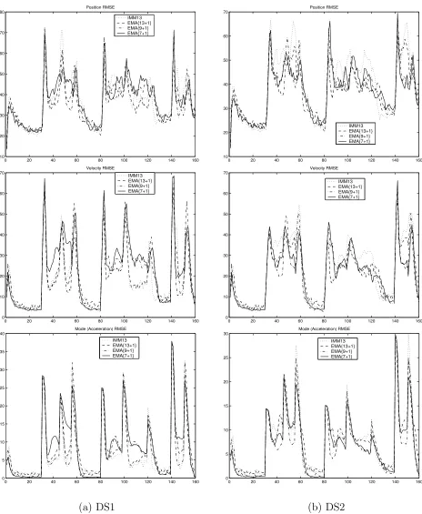
Results over 100 Monte Carlo runs of DS1 and DS2 are plotted in Figure 3.3. It is seen
first that EMA-A{13+1}in both scenarios (and in all other simulated scenarios as well, not
shown) outperforms the remaining algorithms, in particular the fixed-grid IMM13. The
com-parative results between IMM13 on the one hand and EMA-A{9+1}(EMA-A{7+1}) on the
other are scenario dependent. While IMM13 provides less biased steady-state errors in DS1,
EMA-A{9+1} and EMA-A{7+1} give better accuracy for almost all jumps in DS2. This
is due to the fact (mentioned before) that for IMM13, DS1 and DS2 represent respectively
easy and difficult scenarios, regarding the closeness of the true acceleration to the fixed-grid
values. The EMA algorithms are less scenario-dependent.
Results over 500 runs of the random scenario are given in Figure 3.4. Clearly all EMA
designs provide better “overall accuracy”. What is somewhat surprising is the negligible
difference between EMA-A{13+1}and the two other EMA designs, which have fewer models.
A possible explanation is that the modal estimate provides a good “coverage” of the whole
continuous region of possible (simulated) accelerations, even when the number of the fixed
0 20 40 60 80 100 120 140 160 10 20 30 40 50 60 70
80 Position RMSE
IMM13 EMA{13+1} EMA{9+1} EMA{7+1}
0 20 40 60 80 100 120 140 160
10 20 30 40 50 60
70 Position RMSE
IMM13 EMA{13+1} EMA{9+1} EMA{7+1}
0 20 40 60 80 100 120 140 160
0 10 20 30 40 50 60
70 Velocity RMSE IMM13
EMA{13+1} EMA{9+1} EMA{7+1}
0 20 40 60 80 100 120 140 160
0 10 20 30 40 50 60
70 Velocity RMSE
IMM13 EMA{13+1} EMA{9+1} EMA{7+1}
0 20 40 60 80 100 120 140 160
0 5 10 15 20 25 30 35
40 Mode (Acceleration) RMSE
IMM13 EMA{13+1} EMA{9+1} EMA{7+1}
0 20 40 60 80 100 120 140 160
0 5 10 15 20 25
30 Mode (Acceleration) RMSE
IMM13 EMA{13+1} EMA{9+1} EMA{7+1}
(a) DS1 (b) DS2