Vol.7 (2017) No. 4-2
ISSN: 2088-5334
Forecasting Crude Oil Prices Using Discrete Wavelet Transform with
Autoregressive Integrated Moving Average and Least Square Support
Vector Machine Combination Approach
Nurull Qurraisha Nadiyya Md-Khair
#, Ruhaidah Samsudin
#, Ani Shabri
*#
Department of Software Engineering, Faculty of Computing, Universiti Teknologi Malaysia 81310 Johor Bahru, Johor, Malaysia
E-mail: [email protected], [email protected] *
Department of Science Mathematics, Faculty of Science, Universiti Teknologi Malaysia, 81310 Johor Bahru, Johor, Malaysia E-mail: [email protected]
Abstract— In this paper, a hybrid time series forecasting approach is proposed consisting of wavelet transform as the data
decomposition method with Autoregressive Integrated Moving Average (ARIMA) and Least Square Support Vector Machine (LSSVM) combination as the forecasting method to enhance the accuracy in forecasting the crude oil spot prices (COSP) series. In brief, the original COSP is divided into a more stable constitutive series using discrete wavelet transform (DWT). These respective sub-series are then forecasted using ARIMA and LSSVM combination method, and lastly, all forecasted components are combined back together to acquire the original forecasted series. The datasets consist of monthly COSP series from West Texas Intermediate (WTI) and Brent North Sea (Brent). To evaluate the effectiveness of the proposed approach, several comparisons are made with the single forecasting approaches, a hybrid forecasting approach and also some existing forecasting approaches that utilize COSP series as the dataset by comparing the Mean Absolute Error (MAE) and Root Mean Square Error (RMSE) acquired. From the results, the proposed approach has managed to outperform the other approaches with smaller MAE and RMSE values which signify better forecasting accuracy. Ultimately, the study proves that the integration of data decomposition with forecasting combination method could increase the accuracy of COSP series forecasting.
Keywords— autoregressive integrated moving average (ARIMA); least square support vector machine (LSSVM); discrete wavelet
transform; hybrid forecasting method; crude oil spot prices.
I. INTRODUCTION
Crude oil is produced from fossil fuels which compose of hydrocarbon deposits and other organic materials. Crude oil price presents a significant part in the global economy, and its fluctuation is very important for investors and financial practitioners [1]. It is widely utilized in most of the goods manufacturing sector and makes up approximately two-thirds of the world’s energies [2]. Some of the final products are diesel, gasoline, heating oil, lubricant and other forms of petrochemicals. Petrol or also known as gasoline is one of the most important liquids derived from petroleum which is used mainly as fuel for automobiles and other kinds of vehicles powered by internal combustion engine. Changes in crude oil prices can lead to a major impact on global economic movement [3]. For that particular reason, the understanding of petroleum markets is very crucial. One way of doing so is to use time series forecasting methods that are
proposed and proven by many studies. The main objective of time series forecasting is to construct a model that can benefit from the past information to predict the forthcoming events [4].
Autoregressive integrated moving average or ARIMA is a popular model which is applied in time series prediction. It is derived based on the single models namely autoregressive (AR), the moving average (MA) and the consolidation of AR and MA, namely ARMA model [8]. ARMA model is applied mostly in stationary forecasting data series. In the case of non-stationary data series, it is firstly adjusted to be stationary using d which represents the number of difference involved, consequently forming ARIMA. ARIMA model is generally represented by the value (p, d, and q). p defines the number of autoregressive terms and q defines the number of moving average term. Meanwhile, d value is the one that differentiates ARIMA model and ARMA model. It denotes the different order for non-stationary time series.
Least square support vector machine or LSSVM is an alternative to the standard SVM which can be used to analyse the data through classification or regression method. Suykens et al. [9] proposed the method to address short-term load prediction problems. LSSVM is an alteration of SVM model with an extra advantage where it only needs to solve a set of linear equations, rather than quadratic programming which is much easier and computationally simpler. LSSVM method utilizes equality constraints instead of inequality constraints and adopts the least square linear system as its loss function, making it computationally attractive and also has good convergence and high precision. LSSVM is an appropriate method to be applied in time series forecasting because it is a type of Artificial Intelligence (AI) method. An AI-based method models the human mind in problem-solving, therefore it can be used for complex real-world problems [10]. The application of LSSVM has been a success and proven effective in assorted fields [11]-[13].
A lot of methods have been applied to crude oil spot prices (COSP) series forecasting. One of the single methods involved is autoregressive integrated moving average (ARIMA) method which is utilized in performing COSP series forecasting [14]. In this study, the researchers develop an ARIMA model for forecasting the monthly crude oil production in Malaysia. They claimed that the model of (1,0,0) acquired during the empirical study can be used to obtain future forecasts. Unfortunately, COSP series contains volatility, nonlinearity, and irregularity while single forecasting methods can only produce satisfying results when the data series is linear or almost linear [1]. To overcome this problem, researchers propose hybrid methods using data decomposition to enhance the forecasting accuracy. An example of a hybrid method used in forecasting COSP is based on empirical mode decomposition (EMD) which is used for decomposition, feed-forward neural network (FNN) used for prediction and adaptive linear neural network (ALNN) used for assembling [15]. Based on the experiment, they conclude that their proposed hybrid method using data decomposition has performed better than the other methods used as a comparison. Despite that, a suitable data decomposition technique must be carefully inspected before combining with any forecasting method to ensure that good forecasting results can be achieved. Recently, a hybrid forecasting method that integrates data decomposition method with a combination of multiple forecasting models has been proposed [16]. In the study, the researchers come up with the
effort to tackle the problem of prediction performance of the selected individual forecasting approaches which are ARIMA, SVM, Extreme Learning Machine (ELM) and LSSVM. The proposed approach which combines selected forecasting models is proven to be more effective than when they are applied individually or when they are applied with data decomposition using EWT.
The aim of this paper is to propose a discrete wavelet transform (DWT) – ARIMA and LSSVM combination approach to enhance the accuracy of COSP series forecasting. The proposed approach consists of three crucial steps which are (1) breaking down the original COSP series into sub-series via DWT, (2) forecasting using the ARIMA and LSSVM forecasting methods (3) combining the output from each sub-series into the original COSP series by applying the inverse wavelet transform. Several public datasets of COSP from West Texas Intermediate (WTI) and Brent North Sea (Brent) are used in this particular study. To evaluate the effectiveness of the proposed approach, it is compared with the single forecasting approaches, a hybrid forecasting approach and also some existing forecasting approaches by manipulating the Mean Absolute Error (MAE) and Root Mean Square Error (RMSE) acquired from each approach.
The other parts of the study are shown as follows. Section II presents the methodologies involved in this study. The results and discussion of the experiment are elaborated in Section III. Finally, Section IV concludes the overall analysis.
II. MATERIAL AND METHOD
A. Crude Oil Spot Prices Dataset
The COSP datasets used in this research were taken from U.S. Energy Information Administration website that provides a public dataset for crude oil spot prices. In this research, spot prices of crude oil from WTI and Brent from January 2000 until November 2016 were utilized. WTI, also known as Texas light weight is a grade of crude oil used in benchmarking the oil price. WTI grade is defined as light and sweet because it is low in density and sulphuric content, which is only 0.24 percent. Since WTI crude oil is high in quality and is produced within the Midwest and Gulf Coast regions in the U.S, it is refined mostly in those regions. On the other hand, Brent grade also serves as a major benchmark oil price for worldwide oil purchases. Brent grade contains approximately 0.37 percent of sulphur and is considered as light and sweet, similar to WTI. Brent grade is typically refined in Northwest Europe and is applicable in petrol and middle distillates production. Both datasets of WTI and Brent consist of 202 monthly observations respectively.
B. Discrete Wavelet Transform
ensuing wavelet transform equations were quoted from the study done by Kriechbaumer et al. [7]. A mother wavelet derives each wavelet family by translation and expansion to produce daughter wavelets . The equation is described as follows:
(1)
where the mother wavelet function is represented as , translated by the index of location , which signifies its time domain position, and dilated by the scale index , that interprets the width of a daughter wavelet.
Using wavelet transform, a time series is displayed in its time-frequency manner which is called wavelet coefficients. There are several forms of recognizable wavelet transform depending on the number of coefficients produced. The most common ones are continuous wavelet transform (CWT), discrete wavelet transform (DWT) and maximum overlap DWT (MODWT). With respect to DWT, only the number of coefficients required to rebuild the original function was created. To accomplish this reduction, the parameters and were discretized to become and
where and are integers. represents the respective level of decomposition where and is the yielded number of decomposition levels. The choice of a wavelet function and number of decomposition level rely upon the type and frequency of the variations that the analyst wishes to capture in a time series [7]. The following formula can be utilized to assist in finding the suitable number of decomposition level for a particular time series data where L represents the decomposition level, and N represents the observation number of a time series data [18].
(2)
In multiresolution analysis (MRA), a time series data is disintegrated using wavelet transform to form a smooth series that holds the smooth coefficients and a group of detail series comprising of detail coefficients . MRA is a design method devised based on the study of orthonormal, compactly supported wavelet bases. The smooth series which is interpreted as a de-noised form of the original time series is the main component of MRA [5], while the detailed series holds the fluctuations contained in this smooth series. Lastly, the reconstruction of the original series can be done by adding up the coefficients of the detailed series and the smooth series using the following equation:
(3)
C. Autoregressive Integrated Moving Average
Autoregressive integrated moving average (ARIMA) is one of the models commonly used in time series forecasting analysis. It is produced from the autoregressive (AR) model, the moving average (MA) model and the combination of AR and MA called ARMA model. The standard formula to
express the current value of time series for AR model of order p, AR is as follows:
(4)
The current value of a time series as current and previous values of random errors which are expressed by the MA can be formulated as:
(5)
Therefore, the general expression for the merged ARMA process can be described as:
(6)
where represents the predicted value, represents the coefficients associated with preceding white noises, serves as a normal white noise process with zero mean and variance , are the former noise terms.
ARMA method can only be utilized if the time series is stationary. Otherwise, if the time series is non-stationary, the d’th difference process is used to transform it to be stationary where the value is usually 0 or 1 and at most 2. As for such case, the ARIMA model can be described as:
(7)
where . Note that the above equation represents a mixed ARMA model if is replaced with so as to say that . The equations above were quoted from an ARIMA study [19]. Fig. 1 shows the flowchart of Box-Jenkins ARIMA model that consists of model identification, parameter estimation and model validation.
D. Least Square Support Vector Machine
LSSVM is an extension of SVM. Consider a set of data , x represents the input vector, y represents the expected output and n represents the data number. The LSSVM estimates the function in the following form: , where the non-linear mapping outlines the input the data into a higher dimensional feature space.
The optimization problem is formulated by minimizing the regular function when LSSVM is used for function estimation [20]. The equation is as follows:
(8)
where is variable and is regularization parameters which are similar parameter C of SVM and used to control function . The LSSVM is defined in its primal weight space by where the parameter of the model is and , is a function that maps input space into a higher dimensional feature space subject to equality constraint:
(9)
where is error variable. After constructing the Lagrange, the solution is obtained to solve optimization problem:
(10)
where represents Lagrange multipliers which can be positive or negative in the LSSVM formulation. Once and are eliminated, the parameter and are obtained with the LSSVM model. The LSSVM classifier is then constructed as follows:
(11)
where is kernel function, is the support value and is a constant. The most favoured kernel function utilized in LSSVM is the Radial Basis Function (RBF) because it has better efficiency compared to other kernels. Furthermore, RBF is proven to be useful in various applications, but for regression, there can be a better choice. Fig. 2 illustrates the development of LSSVM model.
E. Proposed Hybrid DWT – ARIMA and LSSVM Combination Approach
Firstly, the original COSP series were decomposed using DWT to acquire the smooth series and the detailed series. These individual sub-series were then forecasted using the selected time series forecasting methods. On the one hand, the smooth series was forecasted using ARIMA method. For the purpose of fitting the ARIMA in a short time, the fitting
algorithm introduced by Hyndman et al. [21] was utilized. Using this automatic fitting algorithm, a huge number of forecasts can be simulated in lesser time. On the other hand, the remaining three detail series were forecasted using LSSVM. Prior to that, they were pre-processed by observing the PACF graph generated for each detail series to find the most significant lags to be chosen. Finally, all forecasted components were merged together to obtain the prediction of the originating time series. Fig. 3 depicts the framework for the proposed DWT – ARIMA and LSSVM combination approach.
Fig. 2 Development of LSSVM model
Fig. 3 Forecasting framework for proposed DWT – ARIMA and LSSVM combination approach
F. Hybrid DWT – LSSVM Approach
Fig. 4 Forecasting framework for DWT - LSSVM approach
G. Effectiveness Evaluation
To calculate the prediction accuracy of each forecasting approach, the mean absolute error (MAE) and the root mean square error (RMSE) of those approaches were acquired. The computation for MAE was used to show the similarity between predicted and observed values. The calculation is as follows:
(12)
where is the number of the period forecast, is the real price at time and is the forecasted price at time .
The RMSE was utilized in analysing the forecasting result to determine the tendency of the forecasting models to large forecast errors and measure the overall deviation between predicted and observed values using the following equation:
(13)
III.RESULTS AND DISCUSSION
A. Data Division
Categorizing the datasets is important because a portion of them is required for in-sample or training data while another portion will be used as out-of-sample or testing data. Training data is manipulated to train and develop the forecasting model while testing data is treated as future data that needs to be predicted for the purpose of evaluating the predicting power of a certain forecasting model. The proportion used in this research experiment is agreed to be 80 percent training data and the remaining 20 percent for testing data. Fig. 5 and Fig. 6 show the graph of WTI and Brent monthly COSP from January 2000 to November 2016 respectively. x-axis represents the month while the y-axis represents the price per barrel (USD). From both graphs, it can be observed that the price series are volatile, non-linear, and irregular in terms of its fluctuation.
B. Data Decomposition
For the proposed hybrid DWT – ARIMA and LSSVM combination approach and hybrid DWT – LSSVM approach, the price series are firstly broken down by applying DWT. For decomposition phase, Equation 2 is utilized to the total observation of the data series, and the optimal number of decomposition for both datasets are three-level decomposition. To support this decision, many researchers
have also stated that by using this decomposition level, the description of the price series is more meaningful and thorough, resulting in good forecasting results for non-stationary time series [17], [22]-[24]. Daubechies wavelet function with order 5 is chosen because they present an appropriate trade-off between wave-length and smoothness [17]. Subsequently, the original price series is decomposed into one smooth series and three detail series as shown in Fig. 7. This figure shows the DWT decomposition for WTI dataset. DWT decomposition for Brent is not shown because they are much similar.
Fig. 5 Monthly dataset for WTI COSP
Fig. 6 Monthly dataset for Brent COSP
Fig. 7 Decomposed wavelets for WTI dataset of one smooth series & three detail series
C. ARIMA Model Construction
are not shown because they are much similar. If the ACF graph cuts off rapidly, the prices series is considered stationary. On the contrary, the price series is considered non-stationary if the ACF graph dies down extremely slow [3]. From Fig. 8, it can be noticed that the ACF graph dies down very gently, concluding that the in-sample data is non-stationary. Therefore, differencing needs to be done by using ARIMA model since it is the more appropriate method to handle non-stationary data series.
Fig. 8 ACF (left) and PACF (right) of WTI monthly in-sample data
By applying the automatic fitting algorithm which includes model identification, estimation, and validation, the construction of the time series model is done with the support of a software environment named R using the packages “forecast” and “tseries”. From the result generated, the most fitted model for WTI and Brent Monthly in-sample prices series is ARIMA (1, 1, 0) and ARIMA (0, 1, 1) respectively. From Fig. 9, it can be noticed that the ACF residuals cut off from one lag, hence concluded that the model fits the data appropriately [14]. Validation test which is proposed by Ljung et al. [25] is also illustrated in the result. This model is employed to forecast the out-of-sample data to evaluate the efficacy of the constructed model. The entire ARIMA model construction steps discussed earlier serve as the single forecasting approach for ARIMA.
Fig. 9 Model verification created from R software environment
D. LSSVM Model Construction
Support Vector Machines (SVM) is a powerful methodology for solving problems in non-linear classification, function estimation and density estimation which has also led to many other recent developments in kernel-based learning method, the one which solves convex optimization problems, typically quadratic programs. LSSVM is a reformulation to the standard SVM. Matlab has the toolbox for LSSVM to compile and test the COSP dataset. The Matlab toolbox is built around a fast LS-SVM training and simulation algorithm to yield good values of forecasting. The procedure for developing the LSSVM forecasting model for WTI and Brent monthly COSP is shown below. The entire LSSVM model construction steps will serve as the single forecasting approach for LSSVM.
1) Input Selection: Raw total monthly datasets from WTI and Brent are prepared to be used in the overall development process of the model network.
2) Lag the Data: Arrange the raw total monthly data of WTI and Brent COSP; start with one lagged data until ten lagged data to forecast.
3) Set the Value of Training Dataset and Testing Datasets: Select 80 percent of training data while 20 percent for testing data.
4) Identify the Function Calls: Verify the function calls with codes tunnelssvm, crossvalidatelssvm, trainlssvm and simlssvm to estimate the generalization performance of the trained model included. The estimation of performance based on a fixed test set is calculated by validation.
5) Determination of LSSVM Model: In order to build up an LSSVM model, we need a parameter gamma which acts as the regularization parameter, determining the trade-off between the fitting error minimization and smoothness. In the common case of the RBF kernel, (sig2) is the bandwidth. The parameters and variables relevant to the LSSVM are passed as one cell. The coding in MATLAB is shown in Fig. 10.
Fig. 10 Coding for determining LSSVM model
6) Pre-processing the Data: By default, the data are pre-processed by application of the function “prelssvm” to the raw data and the function “postlssvm” on the predictions of the model. The coding in MATLAB is shown in Fig. 11.
Fig. 11 Coding for data pre-processing
E. Proposed Hybrid DWT – ARIMA and LSSVM Combination Construction
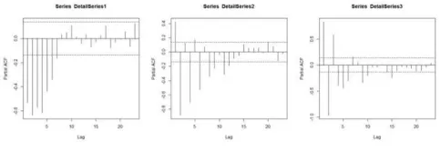
significant lags to be chosen as the inputs to build the LSSVM models. Fig. 12 shows the PACF graph for WTI detail series pre-processing. It is decided that lag 1, 2, 3, 4, 5, and 6 are taken for detail series 1 and detail series 3 while lag 1, 2, 3, 4, and 6 are taken for detail series 2 to equalize the number of lags that will be used as the LSSVM inputs for WTI dataset. Fig. 13 shows the PACF graph for Brent detail series pre-processing. It is decided that lag 1, 2, 3, 4, 5, 6, and 7 are taken for detail series 1 and detail series 3 while lag 1, 2, 4, 5, and 6 are taken for detail series 2 to equalize the number of lags that will be used as the LSSVM inputs for Brent dataset. The process is similar as explained in the LSSVM model construction earlier.
Fig. 12 PACF graph for WTI detail series pre-processing
Fig. 13 PACF graph for Brent detail series pre-processing
After the most appropriate model for each sub-series has been validated, the decomposed sub-series are reconstructed. By using Equation 3 which is the inverse DWT mentioned earlier, the forecasted outputs for the sub-series are converted back into the original price series. MATLAB software is utilized in the decomposition and reconstruction phases.
F. Hybrid DWT – LSSVM Construction
The decomposition procedure and configuration are the same as the one from the proposed hybrid DWT – ARIMA and LSSVM combination approach. The difference between this method and the proposed method is that all decomposed wavelets (one smooth series and three detail series) are forecasted using LSSVM in this method. The pre-processing step in this method is done to all sub-series using PACF graph to determine the most significant lags to be chosen as the inputs to build the LSSVM models. It is decided that lag 1, 2, and 3 are taken for all sub-series following the significant lags from the smooth series to equalize the number of lags that will be used as the LSSVM inputs for WTI and Brent dataset. Once the inputs are finalized, LSSVM is utilized following the same procedure as explained previously in single LSSVM model implementation. Finally, the reconstruction of the decomposed sub-series is done by following the same steps as the proposed approach.
G. Effectiveness Evaluation Result
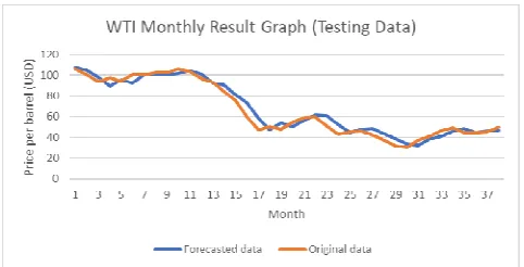
The MAE and RMSE results for the proposed approach, single forecasting approaches and a hybrid forecasting approach for WTI and Brent datasets are shown in Table 1 and Table 2 accordingly. The lower value of MAE and RMSE indicates a higher forecasting accuracy. It can be noticed that the MAE and RMSE results of the hybrid approaches are smaller than the results of the single forecasting approaches. Furthermore, the MAE and RMSE results for the proposed approach are better than the other hybrid approach. Fig. 14 – 17 depict the graphs of the forecasting results for all developed approaches using WTI testing data. Graphs for Brent dataset are not shown because they are quite similar. From the results and graphs, it can be deduced that the proposed approach yields a better and more accurate forecasting result than the single forecasting approaches and the other hybrid approach.
Another comparison is made between the proposed models by other literature that utilized COSP series as the dataset. Table 3 presents the result comparison between the previous works and the proposed approach for testing data. Some existing literature did not utilize MAE or RMSE for result comparison in their paper. Therefore some data might not be available. From the result shown, it can be observed that the proposed approach outperforms all the previous existing models, hence verifying its effectiveness.
TABLEI
MAE &RMSE RESULT COMPARISON BETWEEN DEVELOPED MODELS FOR WTIDATASET
Model Training Data Testing Data MAE RMSE MAE RMSE
ARIMA 3.8134 5.1584 4.0132 4.9741
LSSVM 3.3744 4.4473 4.2174 5.3390
DWT - LSSVM
1.1063 1.4876 1.3130 1.8463
Proposed Approach
0.6043 0.7851 0.9480 1.2143
TABLEII
MAE &RMSE RESULT COMPARISON BETWEEN DEVELOPED MODELS FOR BRENT DATASET
Model Training Data Testing Data MAE RMSE MAE RMSE
ARIMA 4.1293 5.3369 3.9459 5.1377
LSSVM 3.5449 4.6319 4.2527 5.6315
DWT - LSSVM
1.3473 1.7819 1.9168 2.4620
Proposed Approach
0.6833 0.9172 0.9209 1.1909
Fig. 15 WTI monthly result graph (Testing Data) using LSSVM approach
Fig. 16 WTI monthly result graph (Testing Data) using DWT - LSSVM approach
Fig. 17 WTI monthly result graph (Testing Data) using proposed approach
TABLEIII
RESULT COMPARISON BETWEEN PROPOSED HYBRID APPROACH TO THE PREVIOUS WORKS (TESTING DATA)
Model WTI Brent MAE RMSE MAE RMSE
Hybrid ANN model (Amin-Naseri and Gharacheh, 2007)
1.61 1.92 - -
Hybrid AI system
(Wang et al., 2005) - 2.369 - -
SVM (Xie et al.,
2006) - 2.1921 - -
Wavelet Neural Network (Alexandridis and
Livanis, 2008)
1.46 1.84 - -
Proposed
Approach 0.9480 1.2143 0.9209 1.1909
IV.CONCLUSION
This study proposes a hybrid approach in forecasting the COSP series. The proposed approach employs DWT with ARIMA and LSSVM combination to yield a higher forecasting accuracy result. The wavelet transform alters the behaviour of the price series from having unstable variance with outliers to become a set of constitutive series with a more stable variance without outliers. Then, the smooth series is forecasted using ARIMA model while the detailed series are forecasted using LSSVM model. Finally, all sub-series are merged back using inverse wavelet transform to acquire the forecast of the original COSP series. The public datasets of monthly COSP from WTI and Brent are used as the experimental datasets in this research. The experiment is conducted by comparing the MAE and RMSE values of the proposed approach, single forecasting approaches, a hybrid forecasting approach and other literature that utilized COSP series. The final result has managed to verify the effectiveness of the proposed approach by producing more accurate forecasting as compared to other approaches.
In this research, the data are grouped into a ratio of 80% training and 20% testing. Most empirical studies applied the division of 70% vs 30%, 80% vs 20% and 90% vs 10%. It is believed that the more training data are used, the better the accuracy of a forecasting model. Thus, it is suggested for future researchers to divide into how much improvement the division of 70% vs. 30% and 90% vs. 10% could bring compared to 80% vs. 20%. Furthermore, some improvement might be added to the proposed method, and other combination of forecasting models could be utilized to further enhance its accuracy in forecasting crude oil prices. The proposed approach would undergo continuous tests using weekly and daily COSP series datasets for further analysis of its effectiveness.
ACKNOWLEDGMENT
The authors would like to express their deepest gratitude to Research Management Center (RMC), Universiti Teknologi Malaysia (UTM), Ministry of Higher Education Malaysia (MOHE) and Ministry of Science, Technology, and Innovation (MOSTI) for their financial support under Grant Vot 4F875.
REFERENCES
[1] A. Shabri and R. Samsudin, "Daily crude oil price forecasting using hybridizing wavelet and artificial neural network model,"
Mathematical Problems in Engineering, vol. 2014, 2014.
[2] V. G. Azevedo and L. M. Campos, "Combination of forecasts for the price of crude oil on the spot market," International Journal of
Production Research, vol. 54, no. 17, pp. 5219-5235, 2016.
[3] R. Nochai and T. Nochai, "ARIMA model for forecasting oil palm price," in Proceedings of the 2nd IMT-GT Regional Conference on
Mathematics, Statistics and Applications, pp. 13-15, 2006.
[4] W. Waheeb and R. Ghazali, "Chaotic Time Series Forecasting Using Higher Order Neural Networks," International Journal on Advanced
Science, Engineering and Information Technology, vol. 6, no. 5, pp.
624-629, 2016.
[5] P. M. Crowley, "A guide to wavelets for economists," Journal of
Economic Surveys, vol. 21, no. 2, pp. 207-267, 2007.
[6] S. Schlüter and C. Deuschle, Using wavelets for time series
forecasting: Does it pay off? 2010, IWQW discussion paper series.
[7] T. Kriechbaumer, A. Angus, D. Parsons, and M. R. Casado, "An improved wavelet–ARIMA approach for forecasting metal prices,"
[8] V. Ş. Ediger, S. Akar, and B. Uğurlu, "Forecasting production of fossil fuel sources in Turkey using a comparative regression and ARIMA model," Energy Policy, vol. 34, no. 18, pp. 3836-3846, 2006. [9] J. A. Suykens and J. Vandewalle, "Least squares support vector machine classifiers," Neural processing letters, vol. 9, no. 3, pp. 293-300, 1999.
[10] I. Yassin, M. A. Khalid, S. Herman, I. Pasya, N. Ab Wahab, and Z. Awang, "Multi-Layer Perceptron (MLP)-Based Nonlinear Auto-Regressive with Exogenous Inputs (NARX) Stock Forecasting Model," International Journal on Advanced Science, Engineering
and Information Technology, vol. 7, no. 3, pp. 1098-1103, 2017.
[11] M. Afshin, A. Sadeghian, and K. Raahemifar, "On efficient tuning of LS-SVM hyper-parameters in short-term load forecasting: A comparative study," in Power Engineering Society General Meeting,
2007. IEEE, pp. 1-6, 2007.
[12] T. Van Gestel, J. A. Suykens, D.-E. Baestaens, A. Lambrechts, G. Lanckriet, B. Vandaele, B. De Moor, and J. Vandewalle, "Financial time series prediction using least squares support vector machines within the evidence framework," IEEE Transactions on neural
networks, vol. 12, no. 4, pp. 809-821, 2001.
[13] A. Shabri and Suhartono, "Streamflow forecasting using least-squares support vector machines," Hydrological Sciences Journal, vol. 57, no. 7, pp. 1275-1293, 2012.
[14] N. M. Yusof, R. S. A. Rashid, and Z. Mohamed, "Malaysia crude oil production estimation: an application of ARIMA model," in Science
and Social Research (CSSR), 2010 International Conference on, pp.
1255-1259, 2010.
[15] L. Yu, S. Wang, and K. K. Lai, "Forecasting crude oil price with an EMD-based neural network ensemble learning paradigm," Energy
Economics, vol. 30, no. 5, pp. 2623-2635, 2008.
[16] J. Wang and J. Hu, "A robust combination approach for short-term wind speed forecasting and analysis–Combination of the ARIMA (Autoregressive Integrated Moving Average), ELM (Extreme Learning Machine), SVM (Support Vector Machine) and LSSVM
(Least Square SVM) forecasts using a GPR (Gaussian Process Regression) model," Energy, vol. 93, pp. 41-56, 2015.
[17] A. J. Conejo, M. A. Plazas, R. Espinola, and A. B. Molina, "Day-ahead electricity price forecasting using the wavelet transform and ARIMA models," IEEE transactions on power systems, vol. 20, no. 2, pp. 1035-1042, 2005.
[18] V. Nourani, M. T. Alami, and M. H. Aminfar, "A combined neural-wavelet model for prediction of Ligvanchai watershed precipitation,"
Engineering Applications of Artificial Intelligence, vol. 22, no. 3, pp.
466-472, 2009.
[19] W.-c. Wang, K.-w. Chau, D.-m. Xu, and X.-Y. Chen, "Improving forecasting accuracy of annual runoff time series using ARIMA based on EEMD decomposition," Water Resources Management, vol. 29, no. 8, pp. 2655-2675, 2015.
[20] M. Espinoza, J. A. Suykens, and B. De Moor, "Load Forecasting Using Fixed-Size Least Squares Support Vector Machines," in
IWANN, pp. 1018-1026, 2005.
[21] R. J. Hyndman and Y. Khandakar, Automatic time series for
forecasting: the forecast package for R. 2007: Monash University,
Department of Econometrics and Business Statistics.
[22] N. Amjady and F. Keynia, "Day ahead price forecasting of electricity markets by a mixed data model and hybrid forecast method,"
International Journal of Electrical Power & Energy Systems, vol. 30,
no. 9, pp. 533-546, 2008.
[23] J. Hu and J. Wang, "Short-term wind speed prediction using empirical wavelet transform and Gaussian process regression,"
Energy, vol. 93, pp. 1456-1466, 2015.
[24] Z. Tan, J. Zhang, J. Wang, and J. Xu, "Day-ahead electricity price forecasting using wavelet transform combined with ARIMA and GARCH models," Applied Energy, vol. 87, no. 11, pp. 3606-3610, 2010.