Cost Control Development under Stochastic Performance Control

(1)

Published online February 20, 2013 (http://www.sciencepublishinggroup.com/j/ijefm) doi: 10.11648/j.ijefm.20130101.17

Cost control development under stochastic performance

control

Milad Eghtedari Naeini

1,2,*

1

Civil Engineering Department, Pardis, Iran

2

Pardis Islamic Azad University, Pardis, Iran

Email address:

[email protected] (M. E. Naeini)

To cite this article:

Milad Eghtedari Naeini. Cost Control Development under Stochastic Performance Control, International Journal of Nutrition and Food Sciences. Vol. 1, No. 1, 2013, pp. 54-60. doi: 10.11648/j.ijefm.20130101.17

Abstract:

In this research, a model to forecast project’s cost will be presented with due attention to performance time and cost of the project, based on Earned Value Management (EVM) and with regarding real circumstances caused by uncertain-ties, risk factors and using simulation methods. All the uncertainties will be related to cost of work packages as well as its changes over time by probability distribution functions. Probabilistic distribution functions will be determined based on existing information obtained from previous projects and experts’ opinion. In this model, project’s activities will be classified to subgroups calling control accounts. Each of them has a controlling limit to control project’s performance. Then, using simulation methods, stochastic s-curve for each control account will be determined to clarify project stochastic s-curve from total of these s-curves. When a percentage of the project has been performed, using modern methods of Earned Value Management, the performance of the project will be measured, therefore, it will be possible to adjust probability distribution functions and forecast the future performance of the project using simulation model of Monte Carlo.

Keywords:

Monte Carlo Method, Probabilistic Model, Project Forecasting, Stochastic S-Curve, Project Monitoring

1. Introduction

At the beginning of a project, it is necessary to have re-liable forecasts because of existence of naturally risk fac-tors even when there is a detailed plot; these facfac-tors may affect actual performance of the project. Therefore, a project manager should constantly seek leading indices for potential problems to have an appropriate performance at suitable time. Current deviation of the plan functions as an early index of the potential deviation of duration and final cost of project of its purposes.

To control project’s performance is necessary not only for supervision on time and cost variance of the actual project progress, but also it is important for suitable deter-mination of the actual project status based on absolute forecast of final performance of the project. Such forecasts are vital for the project’s manager to know if corrective actions are needed to minimize expected variances of scheduled performance.

Forecast of duration and final cost of the project will be done using two different approaches: deterministic and probabilistic. In the deterministic approach, estimation of time and final costs will be determined considering the

most likely time and cost for each activity. However, in the probabilistic approach, time estimation and planned costs will be determined based on the variability of time and cost distribution for each activity [1].

The final purpose of project performance forecast is to have decision-makers in an appropriate situation achieved from giving them improved and objective pre-awareness; though the experiences of actual performance which might be the most objective and certain information resource for forecasted performances, is limited at the beginning of the project. Therefore, the biggest challenge in forecasting project’s performance is to have a subjective judgment and use prior knowledge to overwhelm the lack of performance experiences achieved to be applied in first phases of the project [2].

The aim of this research is to present a probabilistic model to forecast and control the performance of the project. For this purpose, there are four steps as follows:

• Classifying activities based on their working field in subgroups called control accounts.

• Determining base cost distribution for each activity and escalation cost distribution function for each control account

(2)

• Controlling and update cost baseline using earned value management

Finally, the application of the model will be shown by giving an example.

2. Probabilistic Approach of the Cost

Baseline

Simulation approach is used to produce the stochastic S-curves (SS-curves) which are based on defined variability in duration and cost of the individual activities in process. SS-curves provide probability distributions of required time and budget to complete the project in its middle points [3]. General process of the method to determine distribution of time and cost includes three steps: 1) to produce primary distribution of model’s parameters; 2) to improve model’s parameters based on reported data; 3) to use the improved model to forecast performance [4]. Kim and Reinschmidt (2011) suggested a probabilistic cost forecasting method using Bayesian inference and the Bayesian model averaging technique [5]. Lee et al (2012) proposed the system that assigns probability distribution functions of historical ac-tivity durations to activities, computes the deterministic and stochastic project cashflows, and estimates the best-fit probability distribution functions of overdraft and net profit of a project [6].

At first, to guess the cost of each activity a probability distribution function is supposed and the time for each ac-tivity is considered as a certain and the most likely value. Then, using simulation model of Monte Carlo, distribution of the total cost of the project is estimated. According to Central Limit Theorem, distribution of final cost is normal.

Though SS-curve does not resolve the basic problem of inability in estimation, it is preferred over deterministic S-curve for providing information according to the probable output of the project at different phases of project’s progress [7].

3. Approaches to Measure Project

Per-formance

Approaches to follow the performance are divided into two main groups: (1) Progress Based S-Curve; (2) Time Based S-Curve.

In Progress Based S-Curve, the progress is generally measured according to the amount of completed work not the time taken to finish it. The percentage of the planned work done (progress) is considered as an independent vari-able for being dependent only on the project scope (which is one for actual and planned performance), then time and cost are regarded as dependent variables of progress [8].

Time Based S-Curve is divided into two approaches of EVM and Work/Schedule/Cost/Integrated; in both of them time is independent variable and cost and progress are in-dependent ones. In integrated approach, both cumulative cost and progress are shown in a diagram based on time;

generally, progress (the amount of the work done) is deter-mined based on budget which is measured on the basis of cost, time-worker or physical volume of the work. One of the advantages of this approach is showing progress and cost in one diagram [9].

Earned value management is a valuable methodology in analysis and control of project’s performance. By integra-tion of dimensions of time, cost and scope, the obtained value makes exact measurement of projects’ progress poss-ible and paves the way to on time decision to embark on improving measures. Of course, the focus is mainly on management of costs; even timing indices are calculated on the basis of the costs [10].

4. Developing Probabilistic Approach of

Cost Baseline

In present model, cost distribution functions are divided into two distribution function. The first distribution is de-termined on the basis of the rate of contractor’s productivi-ty in each activiproductivi-ty and is allocated to each activiproductivi-ty which is started at the beginning of the work and called ‘base cost distribution’. The second distribution is determined on the basis of price change in each activity over time because of environmental factors and is called ‘escalation distribution’. Final price for each activity over time is gained by multip-lying the values obtained from these functions.

In previous models, for each activity, a probability dis-tribution function has been considered; therefore it was impossible to find that changes in costs were because of cost change over time or change of contractor’s productivi-ty in that activiproductivi-ty. Further, to define a distribution for long term activities is accompanied with troubles in cost forecast. Considering that the cost of these activities will be with a lot of changes over time, the range of probability distribu-tion funcdistribu-tion for these activities is more extent. It causes that the cost of a part of project which is done sooner to be under the influence of the cost of activity in future raising the price.

4.1. Base Cost Distribution Function of Activities

(3)

The basic advantage of using beta distribution is its abi ity in extensive distribution of forms only with two shape parameters; also, the best distribution is for the time when there is small amount of data [14]. The Beta distribution is a continuous probability distribution on a finite interval A to B with two shape parameters α and β. The Beta probabi ity density function and the Beta function are obtained through Equations 1 and 2 respectively:

1 ( ) ( )

( ; , )

( , ) ( )

x A B x

f x

B B A

A x B

α β

α β α β

− −

=

− ≤ ≤

∫

− ₋ − =1

0

1 1

) 1 ( ) ,

( t t dt

Bα β α β

Shape parameters are determined by collecting data of previous projects and by virtue of Central Limitation the rem [11].

4.2. Escalation Distribution Function of Control Accounts

To model changes of activity costs over time (escalatio we suggest normal distribution. This distribution is dete mined on the basis of the rate of price change of an activity over time. To avoid long calculations, this function is all cated to control accounts instead of each activity. Control accounts are a type of activity grouping each of which b longs to one field. It will be explained in following se tions.

Change in activity cost (escalation) may be created of different factors such as inflation, markets’ conditions, a ticles of risk attribution in the contract, interest, and tax rates [15]. Touran et al (2006) applied normal distribution to forecast escalation rates, too [16]. In suggested model of Touran and Lopez (2006), for each stimulation repetition a random value for escalation is generated for

In latter periods, obtained amounts of previous periods are regarded as mean; however, standard deviation is constant [16]. The proposed system of Hwang et al (2012) can help decision makers in the construction industry deal with changes in economic conditions and design by estimating cost escalations caused by volatile factors such as inflation [17].

In this model, to determine escalation rates of each p riod, first data will be collected from escalation rates of each control account in previous periods. Then, using pr dictor software, escalation rates in next periods will be f recasted. The obtained escalation rates are considered as the mean of normal distributions of each control account.

4.3. Determining Cost of Project

The main purpose of escalation cost modeling is to mo el probabilistic escalation for each control account and f nally all the constructing project. This section consists of three steps: 1) to determine base coat distribution for each control account, 2) to determine distribution of escalation rate, 3) to stimulate cost distribution of escalated project.

The basic advantage of using beta distribution is its abil-ity in extensive distribution of forms only with two shape

meters; also, the best distribution is for the time when ]. The Beta distribution is uous probability distribution on a finite interval A to B with two shape parameters α and β. The Beta probabil-ity densprobabil-ity function and the Beta function are obtained through Equations 1 and 2 respectively:

1 1

1

1 ( ) ( )

( )

x A B x

B A

α β

− −

+ −

− −

− (1)

dt (2)

Shape parameters are determined by collecting data of previous projects and by virtue of Central Limitation

theo-Escalation Distribution Function of Control Accounts

To model changes of activity costs over time (escalation), we suggest normal distribution. This distribution is deter-mined on the basis of the rate of price change of an activity over time. To avoid long calculations, this function is

allo-trol accounts instead of each activity. Conallo-trol a type of activity grouping each of which be-longs to one field. It will be explained in following

sec-Change in activity cost (escalation) may be created of different factors such as inflation, markets’ conditions,

ar-act, interest, and tax ]. Touran et al (2006) applied normal distribution ]. In suggested model of Touran and Lopez (2006), for each stimulation repetition a random value for escalation is generated for the first period. In latter periods, obtained amounts of previous periods are andard deviation is constant The proposed system of Hwang et al (2012) can help decision makers in the construction industry deal with in economic conditions and design by estimating tile factors such as inflation

In this model, to determine escalation rates of each pe-riod, first data will be collected from escalation rates of

periods. Then, using pre-dictor software, escalation rates in next periods will be fo-recasted. The obtained escalation rates are considered as the mean of normal distributions of each control account.

e of escalation cost modeling is to mod-el probabilistic escalation for each control account and fi-nally all the constructing project. This section consists of three steps: 1) to determine base coat distribution for each tribution of escalation rate, 3) to stimulate cost distribution of escalated project.

At first step, distribution of base cost for each control account will be obtained. Base cost is estimated cost for each control account with the current price. Distribut base account for each control account is obtained by adding base cost distributions of existing activities in each control account.

In the second step, distribution of escalation rate of co trol account for each period is determined. Using programs for forecasting, the process of escalation rates are dete mined and considered as mean of the normal distribution for each control account in every period.

In the last step, distribution of project’s final cost in each period will be obtained by multiply e

of each control account by base cost distribution for exis ing activities in that control account; figure 1. Developed system utilizes stimulated software to implement stimul tion. All the explained steps above are repeated in the tw steps above for specific times. The repetition number in stimulation stage depends on confidence intervals accepted for the results.

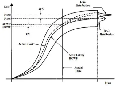
In probabilistic methods, the word ‘variance’ has stati tical meaning and the word ‘variation’ is applied to measure probabilistic performance of the project. In probabilistic approach, cost variation (CV) is the difference between the expected budgeted cost of work p

actual cost of wok performed (ACWP). At

variation (ACV) is evaluated as the difference between expected budget at completion (µBAC) and expected est mate at completion (µEAC), as shown in Figure 1.

Figure 1. Project S

5. Probabilistic Model of Project Pe

formance

5.1. Performance Monitor and Control Functions

In the method of earned value management, early indices of project performance to be bolded provide the need to improvement, including: Schedule

(SPI), this index shows that how actual progression of works is favorite or adverse, and Cost Performance Index (CPI) shows the actual process of cost consuming revealing how this cost was spent favorite or adversely

At first step, distribution of base cost for each control account will be obtained. Base cost is estimated cost for trol account with the current price. Distribution of base account for each control account is obtained by adding base cost distributions of existing activities in each control

In the second step, distribution of escalation rate of con-trol account for each period is determined. Using programs for forecasting, the process of escalation rates are deter-mined and considered as mean of the normal distribution

trol account in every period.

In the last step, distribution of project’s final cost in each period will be obtained by multiply escalation distribution of each control account by base cost distribution for exist-ing activities in that control account; figure 1. Developed system utilizes stimulated software to implement stimula-tion. All the explained steps above are repeated in the two steps above for specific times. The repetition number in stimulation stage depends on confidence intervals accepted

In probabilistic methods, the word ‘variance’ has statis-tical meaning and the word ‘variation’ is applied to measure

abilistic performance of the project. In probabilistic approach, cost variation (CV) is the difference between the pected budgeted cost of work performed (µBCWP) and actual cost of wok performed (ACWP). At-completion cost tion (ACV) is evaluated as the difference between expected budget at completion (µBAC) and expected

esti-pletion (µEAC), as shown in Figure 1.

Project Stochastic S-Curve.

Probabilistic Model of Project

Per-Performance Monitor and Control Functions

(4)

formulas 3 and 4 [10].

BCWS BCWP

SPI= ₍₃₎

ACWP BCWP

CPI= ₍₄₎

Where, BCWS: Budgeted Cost of Wok Scheduled; BCWP: Budgeted Cost of Wok Performed; ACWP: Actual Cost of Wok Performed.

For each control account, indices are allocated. Thre-shold and deviation scope should be determined at the stage of scheduling and used as a guide to test project perfor-mance. Managers and authorities of projects should decide where there is problem and what should be done or sug-gested for that. There are four general responses for devia-tion reports in projects: 1) ignoring that, 2) Funcdevia-tional im-provements, 3) Replanning, 4) redesign of system [18].

After carrying out a percentage of project, future per-formance of project and estimates at completion (EAC) can be forecast using two approaches: 1) future performance does not depend upon past performances and will be done according to predicted schedule, so, to estimate final cost of project, relation 5 will be used. 2) Future performance will be similar to past performance, so, probabilistic estimation of project future performance will be same as past perfor-mance, so, to estimate at completion of the project, rela-tions 6 and 7 are utilized [10].

EAC method in formula 5 accepts actual performance of project which is expressed in actual costs up to now and predicates that all the remained works will be done in bud-geting rate. EAC method in formula 6 supposes that one can expect that the project will continue in future according to what it has experienced in the past. In formula 7, mained work will be done according to efficiency rate re-garding two performance indices, schedule and cost. These two methods suppose negative cost index up to now and the need to provide a scheduled commitment. This method is most useful when the project schedule is a factor impacting the estimate to complete effort. Coefficients a1 and a2 are weighting coefficients of CPI and SPI (such as 50/50 and 20/80 or another relationship) depending on judgment of project management [10].

)

(BAC BCWP

ACWP

EAC= + − ₍₅₎

CPI BAC

EAC= ₍₆₎

(

) (

/ 1 2

)

EAC ACWP

BAC BCWP a CPI a SPI

= +

− +

 

  (7)

One of the useful indices is To-Complete Performance Index (TCPI) which is a calculated plan of cost perfor-mance. It should be obtained for rest of the work to provide a specific management purpose such as budget at comple-tion (BAC) or estimate at complecomple-tion (EAC). If it is ob-served that the budget at completion is not valuable, project manager increases predicted completion estimation for

EAC. To complete performance index can be obtained by dividing the remained work into the remained invest [10].

) /(

)

(BAC BCWP BAC ACWP

TCPI= − − ₍₈₎

Finally, using these two approaches, allocated distribu-tions to activities will be corrected and future performance of the project will be predicted using a new distribution.

5.2. Assigning Control Accounts and Control Limits

To draw an S-curve for the entire project and determine a general performance index for it brings about some prob-lems. This approach causes that performance defects of some of the work packages or sub-projects generalize to the entire project. To resolve this problem, the project is di-vided into sub-groups called control accounts; then, per-formance of each account will be evaluate and control based on its assigned control limit [19].

Activities which are similar in working will be put in groups called control account. These groups or control ac-counts are determined by project manager and can be with-in the framework of Master Format [20]. Then, an S-curve will be drawn for each control account, so, the S-curve of the entire project will be obtained from the total of these S-curves. Further, control limits are specified for each con-trol account. In conclusion, good or bad performance of each control account affects future performance of only the same control account not that of other control accounts. In this model, cost performance indices (CPI) and scheduling performance (SPI) are considered as control limits to eva-luate performance of each control account.

5.3. Specification Limits

Specification limits are the area at both sides of expected baseline showing accepted limitations by the employer for a service or a product [21].

One of the main reasons of limiting uncertainty in some stages is to help imposing pressure on all the members and organization management to understand the importance to differentiate between ‘targets’, which can be desired, ‘ex-pected values’, to predict output, and ‘commitments’ which provide some levels of contingency allowance amount. Targets, expected values and commitments are necessary to be specified regarding their cost, time and all the perform-ing units.

Targets must be realistic to be believed. If optimistic tar-gets are not believed, the expected costs will not be ful-filled. If expected costs and contingency funds are consi-dered as targets, according to Parkinson’s Law, a part of confidence to fulfill expected values has been disregarded in advance. Further, if expected value is considered as the target, even the probability to achieve that will decrease significantly. Generally, values are specified for targets that their probability of fulfillment (or values less than those) is to 20% [22].

(5)

en-forced. The level of commitments is specified based on threatens evaluation and probable opportunities. The level of commitments is normal at maximally

considered 80% [22].

6. Numerical Example

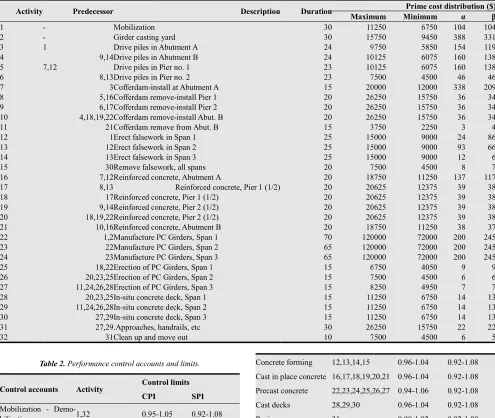
In this section, the mentioned model is p

project with 32 activities as a numeral example. This project is construction of a prestressed concrete girder bridge of three 30 meters spans, with a cast

two middle piers and two abutments [23

is 289 days whose network scheduling is shown in figure 2. Two shape parameters α and β are determined by collecting data of previous projects and fitting distribution to data. By using fitting tool, data distribution will be coincided with

Predecessor Activity

Mobilization

-1

Girder casting yard

-2

Drive piles in Abutment A 1

3

Drive piles in Abutment B 9,14

4

Drive piles in 7,12

5

Drive piles in Pier no. 2 8,13

6

Cofferdam-install at Abutment A 3 7 Cofferdam remove 5,16 8 Cofferdam remove 6,17 9 Cofferdam remove 4,18,19,22 10

Cofferdam remove from Abut. B 21

11

Erect falsework in Span 1 1

12

13

14

Remove falsework, all spans 30

15

Reinforced concrete, Abutment A 7,12

16

8,13 17

Reinforced concrete, Pier 1 (1/2 17

18

Reinforced concrete, Pier 2 (1/2) 9,14

19

Reinforced concrete, Pier 2 (1/2) 18,19,22

20

Reinforced concrete, Abutment B 10,16

21

Manufacture PC Girders, Span 1,2

22

Manufacture PC Girders, Span 2 22

23

Manufacture PC Girders, Span 3 23

24

Erection of PC Girders, Span 1 18,22

25

Erection of PC Girders, Span 2 20,23,25

26

Erection of PC Girders, Span 3 11,24,26,28

27

In-situ concrete deck, Span 1 20,23,25

28

In-situ concrete deck, Span 2 11,24,26,28

29

In-situ concrete deck, Span 3 27,29

30

Approaches, handrails, etc .

27,29 31

Clean up and move out 31

32

Table 2. Performance control accounts and limits

Control accounts Activity Control limits CPI

Mobilization -

Demo-bilization 1,32

0.95-Earth work 2

0.93-Driven piles 3,4,5,6

0.95-Caissons 7,8,9,10,11

0.95-forced. The level of commitments is specified based on threatens evaluation and probable opportunities. The level of commitments is normal at maximally 80-90%, so, we

In this section, the mentioned model is practiced on a project with 32 activities as a numeral example. This project is construction of a prestressed concrete girder bridge of three 30 meters spans, with a cast-in situ deck and [23]. Project duration whose network scheduling is shown in figure 2. ters α and β are determined by collecting data of previous projects and fitting distribution to data. By using fitting tool, data distribution will be coincided with

appropriate beta probability distribution. Maximum and minimum cost for each activity, acc

are specified according to contract’s conditions and project by project management shown in tables 1 and 2

Figure 2. Project network diagram

Table 1. Project activities data.

Duration Description Maximum 11250 30 15750 30

Girder casting yard

9750 24

Drive piles in Abutment A

10125 24

Drive piles in Abutment B

10125 23

Pier no. 1

7500 23

Drive piles in Pier no. 2

20000 15

install at Abutment A

26250 20

Cofferdam remove-install Pier 1

26250 20

Cofferdam remove-install Pier 2

26250 20

Cofferdam remove-install Abut. B

3750 15

Cofferdam remove from Abut. B

15000 25

Erect falsework in Span 1

15000 25

Erect falsework in Span 2

15000 25

ework in Span 3

7500 20

Remove falsework, all spans

18750 20

Reinforced concrete, Abutment A

20625 20

Reinforced concrete, Pier 1 (1/2)

20625 20

18750 20

Reinforced concrete, Abutment B

120000 70

Manufacture PC Girders, Span 1

120000 65

6750 15

Erection of PC Girders, Span 1

7500 15

8250 15

11250 15

situ concrete deck, Span 1

11250 15

26250 30

Approaches, handrails, etc

7500 10

Clean up and move out

Performance control accounts and limits.

Control limits

SPI

-1.05 0.92-1.08

-1.07 0.92-1.08

-1.05 0.92-1.08 -1.05 0.92-1.08

Concrete forming 12,13,14,15

Cast in place concrete 16,17,18,19,20,21 Precast concrete 22,23,24,25,26,27

Cast decks 28,29,30

Paving 31

The mean of escalation distribution for each activity will be determined using predictor software with 5% standard deviation, as shown in table 3

priate beta probability distribution. Maximum and minimum cost for each activity, accounts and control limits fied according to contract’s conditions and project by project management shown in tables 1 and 2

Project network diagram.

Prime cost distribution ($) β α Minimum mum 104 104 6750 11250 331 388 9450 15750 119 154 5850 9750 138 160 6075 10125 138 160 6075 10125 46 46 4500 7500 209 338 12000 20000 34 36 15750 26250 34 36 15750 26250 34 36 15750 26250 4 3 2250 3750 86 24 9000 15000 66 93 9000 15000 6 12 9000 15000 7 8 4500 7500 117 137 11250 18750 38 39 12375 20625 38 39 12375 20625 38 39 12375 20625 38 39 12375 20625 37 38 11250 18750 245 200 72000 120000 245 200 72000 120000 245 200 72000 120000 9 9 4050 6750 6 6 4500 7500 7 7 4950 8250 13 14 6750 11250 13 14 6750 11250 13 14 6750 11250 22 22 15750 26250 5 6 4500 7500

0.96-1.04 0.92-1.08

16,17,18,19,20,21 0.96-1.04 0.92-1.08 24,25,26,27 0.94-1.06 0.92-1.08 0.96-1.04 0.92-1.08 0.98-1.02 0.92-1.08

The mean of escalation distribution for each activity will be determined using predictor software with 5% standard

(6)

Table 3. Control accounts escalation

Control accounts Activity Escalation (day)

1-90 91 Mobilization

-Demobilization 1,32 1.019 1.033

Earth work 2 1.019 1.042

Driven piles 3,4,5,6 1.013 1.030

Caissons 7,8,9,10,11 1.019 1.037

Concrete forming 12,13,14,15 1.018 1.035 Cast in place

con-crete 16,17,18,19,20,21 1.013 1.031

Precast concrete 22,23,24,25,26,27 1.019 1.037

Cast decks 28,29,30 1.018 1.031

Paving 31 1.015 1.016

Monte Carlo stimulation has been applied in this case. After 1000 trails, an estimation of expected cost to complete the project will be obtained. The forecast cost to complete the project is estimated 643987 $ with standard deviation of 627$.

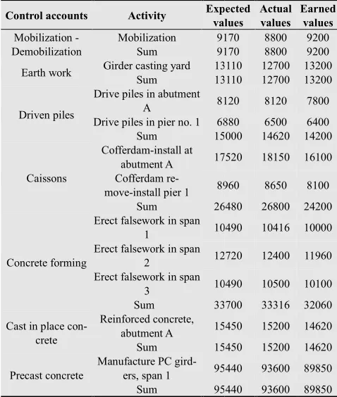
The result of supervising project’s performance at middle point, 100th day by applying the presented model is shown in tables 4 and 5.

Table 4. Project performance monitoring data at day 100

Control accounts Activity Expected values

Mobilization - Demobilization

Mobilization 9170

Sum 9170

Earth work Girder casting yard 13110

Sum 13110

Driven piles

Drive piles in abutment

A 8120

Drive piles in pier no. 1 6880

Sum 15000

Caissons

Cofferdam-install at

abutment A 17520

Cofferdam

re-move-install pier 1 8960

Sum 26480

Concrete forming

Erect falsework in span

1 10490

2 12720

3 10490

Sum 33700

Cast in place con-crete

Reinforced concrete,

abutment A 15450

Sum 15450

Precast concrete

Manufacture PC

gird-ers, span 1 95440

Sum 95440

Table 5. Project performance indices for control accounts at day 100

Control ac-counts

Mobilization -

Demobili-zation Earth work

Driven piles Caissons

Perfor-mance Index

CP

I 1.04 1.03 0.97 0.9

SP

I 1 1 0.95 0.91

Control accounts escalation.

Escalation (day)

-180 181-270 271-289

1.033 1.050 1.066

1.042 1.065 1.087 1.030 1.046 1.063 1.037 1.056 1.075 1.035 1.053 1.071

1.031 1.047 1.062

1.037 1.056 1.075 1.031 1.047 1.062 1.016 1.026 1.036

Monte Carlo stimulation has been applied in this case. After 1000 trails, an estimation of expected cost to complete the project will be obtained. The forecast cost to complete is estimated 643987 $ with standard deviation of

The result of supervising project’s performance at middle point, 100th day by applying the presented model is shown

Project performance monitoring data at day 100.

Expected values

Actual values

Earned values

9170 8800 9200

13110 12700 13200

8120 8120 7800

6880 6500 6400

15000 14620 14200

17520 18150 16100

8960 8650 8100

26480 26800 24200

10490 10416 10000

12720 12400 11960

10490 10500 10100

33700 33316 32060

15450 15200 14620

95440 93600 89850

Project performance indices for control accounts at day 100.

CaissonsConcrete forming

Cast in place

con-crete

Precast con-crete

0.96 0.96 0.96

095 0.95 0.94

As it has been expressed in table 5, control account of ‘Caisson’ is passed the control limit of time and cost pe formance (CPI, SPI). Therefore, this control account has to be improved and rescheduled. If the purpose is to complete the project with initial budget at completion, efficiency (TCPI) should increase to 4% according to formula no. 8. By using formulas 5, 6, 7, the b

estimated. Because this control account has crossed the scheduled performance index (SPI), using formula 7 with a coefficient of 20-80 would be an appropriate method to estimate the cost of this control account for lack of influe of time performance.

Once the project data have been updated with a corrective action, a new project performance forecast could be run in order to evaluate effects in the probabilistic schedule and the revised at-completion performance forecast. If rev at-completion cost and duration variances were improved with respect to the previous forecasted values, the proposed corrective action could be considered acceptable. The co rective performance productivity and the estimate cost forecasts for “Caissons” are shown in Table 6.

performance reports on a project, the project manager u dates the base and escalation distributions and decides whether the project performance is under control and within acceptable control limits so that intervention is

If the project or task is deemed not in control, the project manager needs to identify the causes of the v

necessary actions to get the project back under control and within the acceptable performance limits

Table 6. Performance productivity correction and estimate cost forecasts for “Caissons” at day 100.

TCPI EAC (Eq. 5) EAC (Eq. 6)

1.04 89,583 $ 96,328 $

The graphical representations of forecasting SS are shown in figure 3.

Figure 3. The Project forecasting Stochastic S

5. Conclusions

In this paper cost distribution functions of activities are divided in to two distribution functions: (1) Base Cost Di tribution; (2) Escalation Distribution. Ultima

As it has been expressed in table 5, control account of ‘Caisson’ is passed the control limit of time and cost

per-CPI, SPI). Therefore, this control account has to be improved and rescheduled. If the purpose is to complete the project with initial budget at completion, efficiency (TCPI) should increase to 4% according to formula no. 8. By using formulas 5, 6, 7, the budget at completion can be estimated. Because this control account has crossed the scheduled performance index (SPI), using formula 7 with a 80 would be an appropriate method to estimate the cost of this control account for lack of influence

Once the project data have been updated with a corrective action, a new project performance forecast could be run in order to evaluate effects in the probabilistic schedule and the completion performance forecast. If revised completion cost and duration variances were improved with respect to the previous forecasted values, the proposed corrective action could be considered acceptable. The cor-rective performance productivity and the estimate cost

s” are shown in Table 6. Based on performance reports on a project, the project manager up-dates the base and escalation distributions and decides whether the project performance is under control and within acceptable control limits so that intervention is not necessary. If the project or task is deemed not in control, the project manager needs to identify the causes of the variance and take necessary actions to get the project back under control and within the acceptable performance limits.

ance productivity correction and estimate cost forecasts

EAC (Eq. 6) EAC (Eq. 7)

96,328 $ 80-20 50-50

96,161 $ 95,911 $

The graphical representations of forecasting SS-curves

The Project forecasting Stochastic S-Curves at day 100.

(7)

activity is determined by multiplying base cost distribution by escalation distribution. This fact causes the reason of the change of activity’s cost is discerned whether because of change of cost along the time or change of contractor’s productivity.

The new probabilistic cost forecasting and monitoring method has been developed. It is also an adaptive method that starts with the original estimation of project cost dis-tribution function and adjusts the influence of prior perfor-mance information on prediction as actual perforperfor-mance data accrues.

In this method project activities are classified into sub-groups entitled control accounts. Then, Stochastic S-Curve is obtained for each sub-group and project SS-Curve is obtained by summing sub-groups’ SS-Curve. Thus, project is divided into sub-projects that cause easier and more accurate forecasting and monitoring. Moreover, control limit is determined for each control account to con-trol project performance. If one sub-group needs modifica-tion, it just justifies and it does not affect other sub-groups.

References

[1] K.C. Crandall, and J.C. Woolery, “Schedule development under stochastic scheduling,”Journal of Construction Divi-sion, ASCE, vol.108, pp. 321–329, 1982.

[2] P. Gardoni, K.F. Reinschmidt, and R. Kumar, “A probabilistic framework for Bayesian adaptive forecasting of project progress,” Computer Aided and Civil Infrastruct. Engineer-ing, vol. 22, pp. 182–196, 2007.

[3] G.A. Barraza, E. Back, and F. Mata, “Probabilistic Fore-casting of Project Performance Using Stochastic S Curves,” Journal of Construction Engineering and Management, ASCE, vol. 130, pp. 25-32, 2004.

[4] B.C. kim, and K.F. Reinschmidt, “Probabilistic Forecasting of Project Duration Using Bayesian Inference and the Beta Distribution,” Journal of Construction Engineering and Management, ASCE, vol. 135, pp. 178-186, 2009.

[5] B.C. Kim, and K.F. Reinschmidt, “Combination of Project Cost Forecasts in Earned Value Management,” Journal of Construction Engineering and Management, ASCE, vol. 137, pp. 958–966, 2011.

[6] D. Lee, T. Lim, and D. Arditi, “Stochastic Project Financing Analysis System for Construction,” Journal of Construction Engineering and Management, ASCE, vol. 138, pp. 376–389, 2012.

[7] G.A. Barraza, E. Back, and F. Mata, “Probabilistic Moni-toring of Project Performance Using SS-Curves,” Journal of Construction Engineering and Management, ASCE, vol. 126, pp. 142-148, 2000.

[8] M. Pultar, “Progress-based construction scheduling,” Journal of Construction Engineering and Management, ASCE, vol.

116, pp. 670–688, 1990.

[9] S.A. Ward, and T. Lithfield, Cost control in design and con-struction.McGraw-Hill, New York, NY, USA, 1980. [10] PMI.Practice Standard for Earned Value Management.

Project Management Institute, Inc., Pennsylvania, Pa, USA, 2005.

[11] S.M. AbouRizk, D.W. Halpin, and J.R. Wilson, “Visual Interactive Fitting of Beta Distributions,” Journal of Con-struction Engineering and Management, ASCE, vol. 117, pp. 589-605, 1991.

[12] S.M. AbouRizk, and D.W. Halpin, “Statistical Properties of Construction Duration Data,” Journal of Construction Engi-neering and Management, ASCE, vol. 118, pp. 525-544, 1992.

[13] P. Love, X. Wang, C. Sing, and R. Tiong, “Determining the Probability of Project Cost Overruns,” Journal of Construc-tion Engineering and Management, ASCE, vol. 139, pp. 321–330, 2013.

[14] A. Touran, M. Atgun, and I. Bhurisith, “Analysis of the United States Dept. of Transportation prompt pay provisions,” Journal of Construction Engineering and Management, ASCE, vol. 130, pp. 719–725, 2004.

[15] A.S. Hanna, and A.N. Blair, “Computerized approach for forecasting the rate of cost escalation,” Proc., Comput. Civ. Build. Tech. Conf., pp. 401–408, 1993.

[16] A. Touran, and R. Lopez, “Modeling Cost Escalation in Large Infrastructure Projects,” Journal of Construction En-gineering and Management, ASCE, vol. 132, pp. 853–860, 2006.

[17] S. Hwang, M. Park, H. Lee, and H. Kim, 2012. “Automated Time-Series Cost Forecasting System for Construction Ma-terials,” Journal of Construction Engineering and Manage-ment, ASCE, vol. 138, pp. 1259–1269, 2012.

[18] H. Kerzner, Project Management: A Systems Approach to Planning, Scheduling, and Controlling. 10th ed., John Wiley & Sons, New york, NY, USA, 2009.

[19] M. Eghetdari Naeini, and G. Heravi, “Probabilistic Model Development for Project Performance Forecasting,” World Academy of Science, Engineering and Technology, vol. 58, pp. 396-401, 2011.

[20] CSC., CSI, MASTERFORMAT. The Construction Specifi-cations Institute and Construction SpecifiSpecifi-cations Canada, Alexandria, VA, USA, 2004.

[21] PMI, A guide to the project management body of know-ledge.4thed., Project Management Institute Inc., Pennsylva-nia, Pa, USA, 2008.

[22] C. Chapman, and W. Ward, Project Risk Management Processes, Techniques and Insights. 2nd ed. , John Wiley & Sons, New york, NY, USA, 2003.