Volume 21 Volume 21, 2016 Article 7 2016
Regularization Methods for Fitting Linear Models with Small
Regularization Methods for Fitting Linear Models with Small
Sample Sizes: Fitting the Lasso Estimator using R
Sample Sizes: Fitting the Lasso Estimator using R
W. Holmes FinchMaria E. Hernandez Finch
Follow this and additional works at: https://scholarworks.umass.edu/pare Recommended Citation
Recommended Citation
Finch, W. Holmes and Finch, Maria E. Hernandez (2016) "Regularization Methods for Fitting Linear Models with Small Sample Sizes: Fitting the Lasso Estimator using R," Practical Assessment, Research, and Evaluation: Vol. 21 , Article 7.
DOI: https://doi.org/10.7275/jr3d-cq04
Available at: https://scholarworks.umass.edu/pare/vol21/iss1/7
This Article is brought to you for free and open access by ScholarWorks@UMass Amherst. It has been accepted for inclusion in Practical Assessment, Research, and Evaluation by an authorized editor of ScholarWorks@UMass Amherst. For more information, please contact [email protected].
A peer-reviewed electronic journal.
Copyright is retained by the first or sole author, who grants right of first publication to Practical Assessment, Research & Evaluation. Permission is granted to distribute this article for nonprofit, educational purposes if it is copied in its entirety and the journal is credited. PARE has the right to authorize third party reproduction of this article in print, electronic and database forms.
Volume 21, Number 7, May 2016 ISSN 1531-7714
Regularization Methods for Fitting Linear Models with Small
Sample Sizes: Fitting the Lasso Estimator using R
W. Holmes Finch, Ball State University Maria E. Hernandez Finch, Ball State University
Researchers and data analysts are sometimes faced with the problem of very small samples, where the number of variables approaches or exceeds the overall sample size; i.e. high dimensional data. In such cases, standard statistical models such as regression or analysis of variance cannot be used, either because the resulting parameter estimates exhibit very high variance and can therefore not be trusted, or because the statistical algorithm cannot converge on parameter estimates at all. There exist an alternative set of model estimation procedures, known collectively as regularization methods, which can be used in such circumstances, and which have been shown through simulation research to yield accurate parameter estimates. The purpose of this paper is to describe, for those unfamiliar with them, the most popular of these regularization methods, the lasso, and to demonstrate its use on an actual high dimensional dataset involving adults with autism, using the R software language. Results of analyses involving relating measures of executive functioning with a full scale intelligence test score are presented, and implications of using these models are discussed.
Linear models, including regression, analysis of variance (ANOVA), and their multivariate extensions are perhaps among the most widely used statistical techniques in the social and behavioral sciences. These methods allow researchers to explore relationships among one or more independent variables and a single dependent variable (in the univariate case). The research literature is replete with examples of researchers using such methods. At the same time, researchers and evaluators in the social sciences are often faced with the need to conduct data analysis in the presence of small sample sizes, particularly when they are working with small or difficult to access populations, such as children of migrant workers, adults with autism, or participants in very resource intensive programs that cannot accommodate large numbers of participants (Schunke, Schottle, & Vettorazzi, 2016; Mathur & Parameswaran, 2015; Garcia-Gomez, Risco, Lopez, Guerrero, & Garcia-Pena, 2014).
Given the widespread popularity of linear models, coupled with the potential for problems fitting them in the context of high dimensional data, the purpose of the current manuscript is to describe and to demonstrate some alternatives for fitting linear models when the number of independent variables is nearly as large as, or exceeds the total sample size. In particular, we will focus on the lasso estimator, which belongs to a family of statistical modeling procedures known collectively as regularization methods. The lasso has been shown to be effective for fitting linear models with high dimensional data (e.g. Tibshirani, 1996), yielding estimates with low bias and low standard errors. The paper begins with a brief review of the standard linear regression model, after which the lasso estimator is described. Next, a motivating dataset is introduced, and a thorough demonstration of the lasso using the dataset is presented. Finally, implications for use of the lasso in evaluation and research practice are discussed, along with areas for future research.
The linear model
The standard linear regression model can be written as
⋯ (1)
Where
=Dependent variable value for subject i =Independent variable j value for subject i =Intercept
=Coefficient for independent variable j =Error for subject i
The linear model in equation (1) characterizes the relationship between each independent variable, x, with the dependent variable, y, using the coefficients, . In order to obtain the estimates for these coefficients ( ), the familiar least squares (LS) estimator is typically used. LS identifies values that minimize the squared residuals of the regression model in (1), as expressed in equation (2).
∑ (2)
Where
N =Total sample size
⋯
= Sample estimate of model intercept
= Sample estimate of coefficient for independent variable j
Put another way, LS seeks to find the values of and that minimize the squared difference between the actual dependent variable values and the values that the model predicts.
High dimensional data
In some research and evaluation contexts, the number of variables that can be measured (p) approaches, or even exceeds the number of individuals on whom such measurements can be made (N). For example, the number of participants in a summer horse camp for children identified with an emotional disability might be relatively small due to the amount of resources need to accommodate each participant (e.g. Garcia-Gomez, Risco, Lopez, Guerrero, & Garcia-Pena, 2014). At the same time, program evaluators may be able to obtain a relatively large number of cognitive and
affective measurements for each participant, resulting in high dimensional data. The researchers may want to know how scores on these measures change over time, or how one set of measures is related to another set. However, with a limited sample size the standard linear models, such as regression, that would normally be used to address the research questions may not work well. In particular, when used with small sample sizes, such models will yield inflated standard errors for the model coefficient estimates (Bühlmann & van de Geer, 2011). One consequence of these inflated standard errors is a reduction in power, leading the researcher to erroneously conclude that one or more of the independent variables are not related to the outcome of interest, when in fact they are. Furthermore, having a large number of p independent variables relative to N can result in the presence of collinearity, or very strong relationships among the independent variables, leading to biased parameter estimates, as well as the aforementioned highly inflated standard errors (Fox, 2016). When N=p, a linear regression model will provide perfect fit for the data, although it may not be generalizable to a broader sample, as it is essentially overfitting the sample data (Hastie, Tibshirani, & Friedman, 2009). Finally, when p exceeds N, it is simply not possible to obtain LS estimates for the model parameters, and the researcher is not able to address the research questions of interest.
Regularization methods
There exist a number of strategies for researchers to use in dealing with high dimensional data, including variable selection methods (e.g. stepwise regression, best subsets regression), and data reduction techniques (e.g. principal components regression, supervised principal components regression, and partial least squares regression). Prior research has found that, in the presence of high dimensional data, these variable selection methods can produce estimates with inflated standard errors for the coefficients (Hastie, Tibshirani, & Friedman, 2009). Data reduction models largely mitigate this problem, but they do so by combining the independent variables into a small number of linear combinations, making interpretation of results for individual variables somewhat more difficult, and creating an extra layer of complexity in the model as a whole (Finch, Hernandez Finch, & Moss, 2014).
A third family of techniques that has proven useful in the context of high dimensional data involves
alternative parameter estimation algorithms known as regularization, or shrinkage techniques. Whereas variable selection methods such as best subsets and stepwise regression models assign an inclusion weight of either 1 (include the variable in the model) or 0 (exclude the variable from the model), and then separately estimate the value of for the included variables, regularization methods identify optimal values of the such that the most important independent variables receive higher values, and the least important are assigned coefficients at or near 0. Because these estimates are obtained in a single step and do not involve the either/or decision of the variable selection methods described above, the resulting regularized model variances and standard errors do not suffer from the type of inflation inherent with methods such as best subsets and stepwise regression (Hastie, Tibshirani, & Friedman, 2009). In addition, the regularization methods do not combine the independent variables using linear combinations, thereby avoiding the increased complexity associated with approaches such as principal components analysis. A regularization method that has been shown to be effective across a wide range of conditions is the lasso (Tibshirani, 1996). This method has been used successfully in a number of fields including health statistics (e.g., Li, Feng, & Jiang, 2011; Wu, Chen, Hastie, Sobel, & Lange, 2009), economics (e.g. Shcauberger & Tutz, 2015; Fastrich, Pterlini, & Winker (2015); Fan, Lv, & Qi, 2011), and computer science (e.g. Vastrad & Vastrad, 2013; Kakade, Shalev-Schwartz, & Tewari, 2012), but has received relatively little attention in education and psychology.
The lasso
Regularization methods have in common the application of a penalty to the LS estimator described in equation (1). One such approach is the least absolute shrinkage and selection operator (lasso; Tibshirani, 1996). The fitting criterion for the lasso is written as
∑ ∑ (3)
The terms in equation (3) are as defined above, with the addition of the tuning parameter , which is used to control the amount of shrinkage (i.e. the degree to which the relationship of the independent variables to the dependent variable are down weighted or removed from the model). Larger values correspond to greater shrinkage of the model; i.e. a greater reduction
in the number of independent variables that are likely to be included in the final model. On the other hand, a of 0 leads to the LS estimator. Given the goal of minimizing , the parameter estimates will be reduced in size, and some will even be set to 0, while at the same time the predictions ( ) based upon the parameter estimates should be as accurate as possible, meaning that the parameter estimates cannot all be minimized or set to 0. In other words, the goal of the lasso estimator is to eliminate from the model those independent variables that contribute very little to the explanation of the dependent variable, by setting their values to 0, while at the same time retaining independent variables that are important in explaining y.
In discussing the lasso, it is important to note the tradeoff between estimator bias and variance. The least squares estimator is known to have low bias in many situations, but can also have relatively large variance, particularly in the context of high dimensional data; i.e. relatively many predictors and few observations (Loh & Wainwright, 2012). In contrast, the lasso has been found to have somewhat greater bias than the standard least squares estimator, but with lower variance, particularly in the high dimensional case (Hastie, Tibshirani, & Wainwright, 2015). The increased bias associated with the lasso is caused by the fact that, as noted above, the penalty tends to drive the values of the coefficient estimates toward 0. Thus, the lasso values will underestimate to some extent the population parameters. At the same time, the fact that the magnitudes of the estimates are constrained to some extent means that the lasso estimator will also tend to have smaller variance than least squares, and therefore may provide an overall more accurate prediction than the standard least squares estimate, particularly in the presence of small samples (Tibshirani, 1996).
A key aspect of using the lasso is the determination of the optimal value. The most common approach to finding the appropriate tuning parameter value is through the use of cross-validation. With standard cross-validation the researcher divides the full sample into k subsamples using random selection. One of these subsamples is then designated as the training set, and the others are known as the test sets. The lasso is then applied to the training set for a variety of values, and the resulting estimates are applied to each of the test samples in order to obtain predicted values of for
each individual. The mean square error for test set k with tuning parameter value ( ) is then calculated for each of the test samples as
∑
(4)
Where
=Dependent variable value for subject i in test set k Model predicted dependent variable value for subject i in test set k using
The values are then averaged across the K test samples for each value of . The optimal value of
is the one that yields the lowest mean . If the sample is too small to be divided into training and cross-validation samples, a variation called leave-one-out or jackknife cross-validation can be used instead (Efron & Stein, 1981; Tukey, 1958; Quenouille, 1949). With this method, the lasso model is fit to the data leaving out one individual and then applying the cross-validation method described above to compare that individual’s actual and predicted values of y. This individual is then placed back into the sample, another individual is removed, the lasso model fit to the data, and model parameters applied to the data of the newly removed individual in order to obtain a cross validation estimate of the value in equation (4). This approach is repeated for each individual in the sample so that the 〖
is calculated involving all members of the sample. As an example, consider a sample consisting of 10 individuals. The jackknife approach for determining the optimal value of would proceed as follows:
1. Remove person 1 from the dataset and estimate a regression model for a given λ value using the other 9 individuals in the sample.
2. Use the parameter estimates obtained in step 1 to obtain a predicted value of the dependent variable for person 1.
3. Calculate the squared difference between the observed and model predicted dependent variable values for person 1 at the specific value of .
4. Repeat steps 1 through 3 for person 1, using different values of .
5. Repeat steps 1 through 4, removing person 2 from the data and reinserting person 1.
6. Use equation (4) to calculate the MSE for each value of
7. Select the value of that has the smallest value of MSE
Inference for regularization methods
Researchers using regression techniques are typically interested not only in obtaining an estimate of the relationships between the independent and dependent variables, but also in ascertaining whether there is likely to be a relationship among these variables in the population; i.e. whether there is a statistically significant relationship between the independent and dependent variables. The adaptive nature of the regularization approaches makes the question of inference potentially difficult to answer, because the methods are simultaneously engaging in variable selection and parameter estimation (Hastie, Tibshirani, & Wainwright, 2015). In other words, with the lasso variable selection and statistical inference are intertwined, making the determination of statistical significance somewhat difficult. Researchers working on this problem have suggested using a Bayesian approach (Park & Casella, 2008), or the bootstrap (Meinhausen & Bühlmann, 2010) in order to conduct statistical inference for the regularization methods. Both approaches incorporate variable selection with model inference, so that the issue of statistical significance remains intertwined with variable selection.
Work has also been done in the area of post-selection inference for regularization methods. Perhaps the most promising of these approaches is the covariance test (Lockhart, Taylor, Tibshirani, & Tibshirani, 2014). The test is conducted after the optimal value of , and thus the final set of independent variables to be included in the model have been selected. In order to test for the significance of the coefficient associated with independent variable ,, the algorithm first identifies the value of for which
entered the model, which is denoted as . The model parameter estimates at this step are . Next, the independent variables that were included in the model prior to the entrance of for are identified and called . The algorithm then refits the regularized regression model using only the set of independent variables (i.e. excluding ), but using the value of as the regularization parameter. This model yields the parameter estimates . The covariance test is then calculated as
〈 , 〉 〈 , 〉 (5)
Where
〈 , 〉 =Covariance between actual y and model predicted y including variable
〈 , 〉 = Covariance between actual y and model predicted y excluding variable
= Residual sum of squares for the solution with p predictors
is distributed as an F statistic with 2 and N-p degrees of freedom. The covariance test compares the additional amount of variance accounted for by the model when variable is included in the model versus when it is excluded. A statistically significant result for would lead to rejection of the null hypothesis that does not contribute to explaining the dependent variable y.
Empirical example using R
MethodologyIn order to demonstrate the utility of the lasso approach for fitting linear models, data analysis was conducted using an exemplar dataset. The data were collected on 10 adults with autism who were clients of an autism research and service provision center at a large Midwestern university. Adults identified with autism represent a particularly difficult population from which to sample, meaning that quite frequently sample sizes are small. The sample for this analysis was comprised of 10 adults (9 males), with a mean age of 20 years, 2 months (SD=1 year, 9.6 months). Of interest for the current analysis was the relationship between executive functioning as measured by the Delis-Kaplan Executive Functioning System (DKEFS; Delis, Kaplan, & Kramer, 2001) and the full scale intelligence score (FSIQ) on the Wechsler Adult Intelligence Scale, 4th edition (WAIS-IV; Wechsler, 2008). Because of the difficulty in obtaining samples of adults with autism, relatively little work has been conducted with this population regarding the relationship between executive functioning and IQ, although it is known to be particularly relevant for individuals with autism in general (Mclean, Johnson Harrison, Zimak, & Morrow, 2014).
In order to demonstrate the utility of the lasso with small samples, regression models with FSIQ as the
dependent variable, and the 16 DKEFS subscales appearing in Table 1 as the independent variables were fit using each of the regularization methods separately. Analyses were conducted with the glmnet library in the R software package, version 3.11 (R Core Development Team, 2014). Standard least squares regression could not be used in this case, because the number of independent variables exceeded the sample size. In addition, given the small sample size, the leave-one-out cross-validation approach was used to identify the optimal value of . Prior to conducting the analysis, the necessary R libraries must be loaded, using the library command.
library(Scale) library(glmnet)
library(selectiveInference)
The data are then standardized prior to the conduct of the statistical analyses.
#Standardize the variables prior to conducting data analysis# attach(wais_dkefs.final) wais_dkefs.z<‐scale(wais_dkefs.final, center=TRUE, scale=TRUE) dkefs.z<‐ as.matrix(wais_dkefs.z[,2:17]) Results
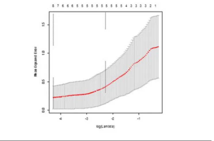
The first step in using the lasso estimator is to determine the optimal value of the tuning parameters. As described above, the optimal value of can be ascertained using leave-one-out cross-validation. Figure 1 displays the leave-one-out cross-validated mean square error (MSE) for the natural log of . Following are the R commands to fit the cross-validated model using the jackknife approach described above, which is called through the use of nfolds= the number of observations in the dataset.
wais_dkefs.z.lasso.cv<‐
cv.glmnet(dkefs.z,wais_dkefs.z[,1], type.measure="mse", nfolds=10) plot(wais_dkefs.z.lasso.cv)
Figure 1. Leave-One-Out Cross-Validation Mean Squared Error by the log of (bottom axis) and the number of non-zero coefficients (top axis)
It is clear that the MSE was smaller for lower values of the regularization parameter. For the lasso estimator, the optimal is the one that minimizes the leave-one-out MSE value calculated using equation (4). In this example, the minimum was determined through leave-one-out cross-validation to be 0.139. While it is not easy to ascertain this minimum value from the figure above, the glmnet R library has a convenient function that will show the value of corresponding to the minimum MSE. This function appears below.
wais_dkefs.z.lasso.cv$lambda.min [1] 0.01394299
In addition, to provide a further demonstration of the relationship between λ and MSE, we fit the model for several values of λ and then calculated the MSE for each. These values appear in Table 1. From these, we can see that larger values of λ were associated with the largest MSE values and declined as λ approached its optimal value of 0.0139, where MSE was minimized. When λ was less than 0.0139, MSE increased once again, as we can see in Table 1. This is the pattern that is demonstrated in Figure 1.
Table 1. MSE by value of for selected MSE 0.0100 0.2402 0.0139 0.2387 0.0180 0.2501 0.1350 0.4891 0.3679 0.9215
For the optimal value, 8 of the 16 predictors were retained in the model, and the R2 value was 0.91; i.e. 91% of the variance in FSIQ was explained by the 8 retained DKEFS variables.
Figure 2 displays the magnitude of the model coefficients on the y-axis for each variable (represented by the individual lines) for each model (represented by the individual panels in the figure), by the magnitude of the log of appearing on the x-axis. The R commands for fitting the lasso model, and then plotting the values of the model coefficients by the log of appears below, followed by the resulting graphical output
wais_dkefs.z.lasso<‐ glmnet(dkefs.z,wais_dkefs.z[,1],alpha= 1, standardize=FALSE, nlambda=100) plot(wais_dkefs.z.lasso, xvar="lambda", label=TRUE, ylab=c("Lasso Coefficient"))
Figure 2. Model Coefficients by Log of Lambda for the Lasso
Larger values of the log of reflect a more severe penalty. From these results it is clear that as the penalty becomes more severe, the number of variables with coefficients near 0 becomes larger as well. Of interest to the researcher is identification of the value that yields the most parsimonious model (i.e. one with as few non-zero coefficients as possible) that also explains as substantial amount of the variance in the dependent
variable as possible. To this end, Figure 3 displays the R2 value (lower x-axis) for each model (panels) by the magnitude of the coefficients (y-axis) and the number of variables included in the model (upper x-axis).
plot(wais_dkefs.z.lasso, xvar="dev", label=TRUE, ylab=c("Lasso
Coefficient"), xlab=c("R Squared"))
Figure 3. Model Coefficients by R2 for Lasso
Clearly, as the number of included variables was greater, so was the R2 value. The key for the researcher using the lasso is to find the optimal tuning parameter values so that a relatively parsimonious model is selected that explains a relatively large amount of variance in the dependent variable. As noted above, this value for was 0.139.
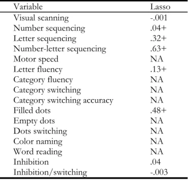
The standardized parameter estimates (i.e. beta weights) for each model appear in Table 2. These are the standardized weights because we first standardized the data prior to fitting the model. Following is the R command to obtain the coefficients for the lasso estimator at the optimal value of .
coef(wais_dkefs.z.lasso.cv,s="lambda.m in")
Table 2. Standardized Model Coefficients for Independent Variables Variable Lasso Visual scanning -.001 Number sequencing .04+ Letter sequencing .32+ Number-letter sequencing .63+ Motor speed NA Letter fluency .13+ Category fluency NA Category switching NA Category switching accuracy NA
Filled dots .48+ Empty dots NA Dots switching NA Color naming NA Word reading NA Inhibition .04 Inhibition/switching -.003
*NA=Variable not selected for inclusion in final model +Statistically significant at =0.05
The optimal lasso model included 8 of the original 16 variables. Variables that were left out of the final model are denoted by NA in the table.
In order to determine which of the DKEFS scores were significantly related to the FSIQ, the covariance test, which was described above, was used. To access this test in R, the slectiveInference library must first be loaded. The following commands can then be employed in order to obtain the results for the covariance tests of the null hypothesis of no relationship with the dependent variable, for each of the independent variables. lasso.sigma<‐ estimateSigma(dkefs.z,wais_dkefs.z[,1] , intercept=FALSE, standardize=FALSE) lasso.beta = coef(wais_dkefs.z.lasso, s=.0139)[‐1] lasso.inference = fixedLassoInf(dkefs.z,wais_dkefs.z[,1] ,lasso.beta,.0139, sigma=lasso.sigma$sigmahat) lasso.inference
The indication of statistical significance for each of the independent variables appears in Table 2, above. Of
the 8 variables that the lasso included in the model, 5 were statistically significantly related to FSIQ (Number sequencing, Letter sequencing, Number-letter sequencing, Letter fluency, and Filled dots), and all had positive coefficients. Thus, higher scores on each of these subscales were associated with higher FSIQ scores. These coefficients are based upon the standardized data, and therefore can be interpreted in the same fashion as are beta weights in traditional regression analysis. For example, a 1 standard deviation increase in the variable Number-letter Sequencing was associated with a 0.63 standard deviation increase in the WAIS score.
Discussion
Researchers working in the social sciences are not infrequently faced with the problem of having to work with small samples. For example, a summer horse camp intervention for children identified with emotional problems might be very resource intensive, so that only a small number of individuals can participate. At the same time, a relatively large number of measurements might be made on each individual (e.g. daily behavior ratings, cognitive assessments throughout the camp, parental ratings at regular intervals), thereby creating a high dimensional dataset in which the number of variables approaches or exceeds the sample size. Whatever the cause, researchers faced with small samples and high dimensional data will find the use of popular statistical techniques, such as regression and ANOVA, to be difficult at best, and impossible at worst, as in the example presented above. In order to use a standard model such as regression in this case, the researcher would either need to make a subjective determination regarding which independent variables to exclude from the analysis, fit several smaller models using subsets of the independent variables, or attempt to collect more data, which may not be feasible. It is in such situations that regularization techniques may be extremely useful.
A word should be given regarding how best to report, in publications, results from studies using the lasso. Of key importance in reporting the results of the lasso is the approach used to determine the optimal value of the tuning parameter, . Therefore, the author will want to include all of the relevant information that led to the selection of this value, such as the graphical presentation of MSE by the log of , as demonstrated in Figure 1 above. In addition, the researcher will also
want to provide the reader with information about the magnitudes of the regression coefficients for the variables by the value of , as in Figure 2, and the proportion of variance explained by models with varying values and numbers of predictors (Figure 3). Both the MSE by and coefficient by graphs provide the reader with a sense for what the optimal tuning parameter value should be, and how this value impacts the results of the analysis. In addition to focusing on , it is also key to present the parameter estimates and hypothesis testing results for the optimal tuning parameter value, as was done in Table 2 above.
Extensions of regularization methods
In addition to regression models such as the one presented above, the lasso can also be used in the context of multivariate data (i.e. more than one dependent variable) such as MANOVA (Ullah & Jones, 2015), logistic regression for categorical dependent variables (Tibshirani, 1996), survival analysis (Tibshirani, 1997), factor analysis (Hirose & Yamamoto, 2015), and cluster analysis (Pan, Shen, & Liu, 2013). While the goals of these various methods are quite different from one another, the underlying regularization methodology is very much the same as for the approaches described here. In all cases, a penalized fitting function is used to ensure that only salient variables are retained in the final model, thereby making accurate parameter estimation more possible than would be the case if all possible variables were used. As was demonstrated above, using such regularization procedures is relatively straightforward in the R software environment, and prior simulation work has shown that the parameter estimates obtained from these models are quite accurate under a variety of circumstances (e.g. Tibshirani, 1996).
In addition to the lasso, other regularization methods have also been suggested for use with high dimensional data. These include the grouped lasso (Yuan & Lin, 2006), in which sets of variables are kept or remove together, the adaptive lasso (Zou, 2006), whereby separate lasso estimators are used in subsequent steps, the Bayesian lasso (Park & Casella, 2008), and the elastic net (Zou & Hastie, 2005), which includes a second tuning parameter in addition to , among others. These additional methods offer alternatives for researchers working with high dimensional data, and continue to be studied by
statisticians in order to better understand their properties across a range of data conditions.
References
Bühlmann, P. & van de Geer, S. (2011). Statistics for High-Dimensional Data: Methods, Theory and
Applications. Berlin: Springer-Verlag.
Dellis, D.C., Kaplan, E., & Kramer, J.H. (2001). Delis-Kaplan Executive Function System (D-KEFS). San Antonio, TX: the Psychological Corporation. Efron, B. & Stein, C. (1981). The Jackknife Estimate of
Variance. The Annals of Statistics, 9(3), 586-596. Fan, J., Lv, J., & Qi, L. (2011). Sparse High-Dimensional
Models in Economics. Annual Review of Economics, 3, 291-317.
Fastrich, B., Paterlini, S., & Winker, P. (2015). Constructing Optimal Sparse Portfolios using Regularization
Methods. Computational Management Science, 12(3), 417-434.
Finch, W.H., Hernandez Finch, M.E., & Moss. (2014). Dimension Reduction Regression Techniques for High Dimensional Data. General Linear Model Journal, 40(2), 1-15.
Garcia-Gomez, A., Risco, M. L., Rubio, J.C., Guerrero, E., & Garcia-Pena, I.M. (2014). Effects of a Program of Adapted Therapeutic Horse-Riding in a Group of Autism Spectrum Disorder Children. Electronic
Journal of Research in Educational Psychology, 12(1), 107-128.
Hastie, T., Tibshirani, R., & Friedman, J. (2009). The Elements of Statistical Learning: Data Mining, Inference, and Prediction. New York: Springer-Verlag.
Hastie, T., Tibshirani, R., & Wainwright, M. (2015). Statistical Learning with Sparsity: The lasso and generalizations. Boca Raton, FL: CRC Press, A Taylor & Francis Group.
Hirose, K. & Yamamoto, M. (2015). Sparse Estimation via Nonconcave Penalized Likelihood in Factor Analysis Model. Statistical Computing, 25, 863-875.
Kakade, S.M., Shalev-Schwartz, S., & Tewari, A. (2012). Regularization Techniques for Learning with Matrices.
Journal of Machine Learning Research, 13, 1865-1880. Li, W., Feng, J., & Jiang, T. (2011). IsoLasso: A Lasso
Regression Approach to RNA-Seq Based Transcriptome Assembly. Journal of Computational Biology, 18(11), 1693-1707.
Lockhart, R., Taylor, J., Tibshirani, R., & Tibshirani, R. (2014). A Significance Test for the Lasso. Annals of Statsitics, 42(2), 413-468.
Loh, P-L. & Wainwright, M.J. (2012). High-Dimensional Regression with Noisy and Missing Data: Provable Guarantees with Nonconvexity. The Annals of Statistics, 40(3), 1637-1664.
McLean, R.L., Johnson Harrison, A., Zimak, E., Joseph, R.M., & Morrow, E.M. (2014). Executive Function in Probands with Autism with Average IQ and their Unaffected First-Degree Relatives. Journal of the American Academy of Child & Adolescent Psychiatry, 53(9), 1001-1009.
Meinhausen, N., & Bühlmann, P. (2010). Stability Selection. Journal of the Royal Statistical Society, Series B, 72(4), 417-473.
Mathur, S., & Parameswaran, G. (2015). Gender Neutrality in Play of Young Migrant Children: An Emerging Trend or an Outlier? American Journal of Play, 7(2), 174-200.
Pan, W., Shen, X., Liu, B. (2013). Cluster Analysis:
Unsupervised Learning via Supervised Learning with a Non-convex Penalty. Journal of Machine Learning Research, 14, 1865-1889.
Park, T. & Casella, G. (2008). The Bayesian Lasso. Journal of the American Statistical Association, 103(482), 681-686. Quenouille, M.H. (1949). Problems in Plane Sampling. The
Annals of Mathematical Statistics, 20(3), 355-375. R Core Development Team. (2015). R: A language and
environment for statistical computing. R Foundation for Statistical Computing, Vienna, Austria.
Schauberger, G. & Tutz, G. (2015). Regularization Methods in Economic Forecasting. In J. Beran, J. Feng, & H. Hebbel (Eds.) Empirical Economic and Financial Research. New York: Springer.
Schunke, O., Schottle, D., Vettorazzi, E. (2016). Mirror Me: Imitative Responses in Adults with Autism. The International Journal of Research and Practice, 20(2), 134-144.
Tibshirani, R. (1997). The Lasso Method for Variable Selection in the Cox Model. Statistics in Medicine, 16, 385-395.
Tibshirani, R. (1996). Regression Shrinkage and Selection via the Lasso. Journal of the Royal Statistical Society, Series B., 58, 267-288.
Tukey, J.W. (1958). Bias and Confidence in Not-quite Large Samples. The Annals of Mathematical Statistics, 29(2), 614-623.
Ullah, I. & Jones, B. (2015). Regularized MANOVA for high-dimensional data. Australian & New Zealand
Journal of Statistics, 57(3), 377-389.
Vastrad & Vastrad, C.M. (2013). Performance Analysis of Regularized Linear Regression Models for Oxazolines and Oxazoles Derivatives Descriptor Dataset.
International Journal of Computational Science and Information Technology, 1(4), 111-123.
Wechsler, D. (2008). Wechsler Adult Intelligence Scale-Fourth Edition. San Antonio, TX: Pearson.
Wu, T.T., Chen, Y.F., Hastie, T., Sobel, E., & Lange, K. (2009). Genome-wide Association Analysis by Lasso Penalized Logistic Regression. Bioinformatics, 25(6), 714-721.
Yuan, M. & Lin, Y. (2006). Model Selection and Estimation in Regression with Grouped Variables. Journal of the Royal Statistical Society, Series B, 68, 49-67.
Zou, H. (2006). The Adaptive Lasso and its Oracle Properties. Journal of the American Statistical Association, 101, 1418-1429.
Zou, H. & Hastie, T. (2005). Regularization and Variable Selection via the Elastic Net. Journal of the Royal Statistical Society, Series B., 67(2), 301-320.
Appendix
R code and output for fitting the lasso and elastic net models for example data Example data file
Y X1 X2 X3 X4 X5 X6 X7 X8 X9 X10 3.741530 0.573051 -0.175230 -1.339954 -0.368095 1.090042 -0.115272 -0.577052 0.425472 0.179867 1.088520 0.100441 1.183853 -0.694153 -0.766538 0.455033 -0.017487 -1.367410 -0.050084 -0.817974 -1.559255 0.579605 2.553595 1.007614 1.543381 0.463916 -0.898300 -0.053513 1.533398 0.180512 0.113829 -0.096545 -0.352276 0.153503 -1.341994 -1.445909 1.730850 1.027419 0.677408 -0.001175 -0.138712 -0.759287 -0.447889 0.483444 1.465349 1.104495 -0.507631 -0.517296 0.242078 0.761720 -1.901134 -2.223851 -0.736562 2.318569 -2.272791 -0.012732 0.111837 -0.846025 0.155868 -0.897112 -1.184396 -0.295120 0.881524 0.966334 -1.903001 1.055233 0.726743 -0.320148 0.297111 0.508650 0.206923 -0.527616 -0.030750 -0.805411 0.766234 0.496932 -0.120334 2.170335 0.068812 1.809094 -0.761952 -2.154671 -0.286850 -0.860617 -0.102291 2.345841 0.284032 0.253651 -1.669843 -1.172163 -1.161900 0.935259 0.858773 -0.271187 -1.231314 -0.238721 -1.086486 0.989511 2.269332 1.009178 1.741643 1.454726 -2.975978 2.920440 -0.798064 0.156104 1.350790 -1.084402 -0.943684 -0.180285
#Read the data from a .dat file, print the data to be sure that it# #was read in
correctly, and create matrices of the independent and#
#dependent variables.#
demo<‐read.table("c:/research/lasso demonstration/demo.dat", header=F)
demo
demo.iv<‐as.matrix(demo[,2:11])
demo.dv<‐as.matrix(demo[,1])
#Cross‐validation to determine optimal value of lambda#
demo.lasso.cv<‐cv.glmnet(demo.iv, demo.dv, type.measure="mse", nfolds=10)
plot(demo.lasso.cv)
demo.lasso.cv$lambda.min
[1] 0.01543617
#Fit the LASSO model and plot coefficient values by log of lambda and R‐square#
demo.lasso<‐glmnet(demo.iv,demo.dv,alpha=1, standardize=FALSE, nlambda=100)
plot(demo.lasso, xvar="lambda", label=TRUE, ylab=c("Lasso Coefficient"))
plot(demo.lasso, xvar="dev", label=TRUE, ylab=c("Lasso Coefficient"), xlab=c("R
#Coefficients for the minimum value of lambda#
coef(demo.lasso.cv, s="lambda.min")
11 x 1 sparse Matrix of class "dgCMatrix" 1 (Intercept) 1.1448974 V2 0.5251900 V3 . V4 ‐0.2920695 V5 . V6 1.3487055 V7 0.6581483 V8 . V9 0.7553453 V10 0.1237440 V11 .
#Conduct post‐selection inference for the lasso#
library(selectiveInference)
lasso.sigma<‐estimateSigma(demo.iv,demo.dv)
lasso.beta = coef(demo.lasso, s=.01543617)[‐1]
#[‐1] leaves out the intercept from inference#
lasso.inference = fixedLassoInf(demo.iv,demo.dv,lasso.beta,.01543617,
sigma=lasso.sigma$sigmahat)
lasso.inference
Call:
fixedLassoInf(x = demo.iv, y = demo.dv, beta = lasso.beta, lambda = 0.01543617, sigma = lasso.sigma$sigmahat)
Standard deviation of noise (specified or estimated) sigma = 0.211
Testing results at lambda = 0.015, with alpha = 0.100
Var Coef Z‐score P‐value LowConfPt UpConfPt LowTailArea UpTailArea 3 ‐0.737 ‐9.449 0.000 ‐0.878 ‐0.602 0.048 0.049 4 ‐0.344 ‐2.900 0.004 ‐0.556 ‐0.142 0.050 0.050 5 1.094 6.652 0.000 0.817 1.397 0.048 0.049 6 0.893 8.074 0.000 0.688 1.087 0.049 0.050 7 ‐0.298 ‐1.645 0.103 ‐0.661 0.102 0.049 0.050 8 0.317 2.177 0.030 0.043 0.564 0.049 0.048 10 ‐0.118 ‐1.317 0.184 ‐0.280 0.109 0.050 0.049
Note: coefficients shown are partial regression coefficients
Citation:
Finch, W. Holmes, & Finch, Maria E. Hernandez (2016). Regularization Methods for Fitting Linear Models with Small Sample Sizes: Fitting the Lasso Estimator using R. Practical Assessment, Research & Evaluation, 21(7). Available online: http://pareonline.net/getvn.asp?v=21&n=7.
Corresponding Author Holmes Finch
George and Frances Ball Distinguished Professor of Educational Psychology Department of Educational Psychology
Ball State University Muncie, IN