R E S E A R C H
Open Access
An analysis on equal width quantization and
linearly separable subcode encoding-based
discretization and its performance resemblances
Meng-Hui Lim, Andrew Beng Jin Teoh
*and Kar-Ann Toh
Abstract
Biometric discretization extracts a binary string from a set of real-valued features per user. This representative string can be used as a cryptographic key in many security applications upon error correction. Discretization performance should not degrade from the actual continuous features-based classification performance significantly. However, numerous discretization approaches based on ineffective encoding schemes have been put forward. Therefore, the correlation between such discretization and classification has never been made clear. In this article, we aim to bridge the gap between continuous and Hamming domains, and provide a revelation upon how discretization based on equal-width quantization and linearly separable subcode encoding could affect the classification performance in the Hamming domain. We further illustrate how such discretization can be applied in order to obtain a highly resembled classification performance under the general Lp distance and the inner product metrics. Finally, empirical studies conducted on two benchmark face datasets vindicate our analysis results.
1. Introduction
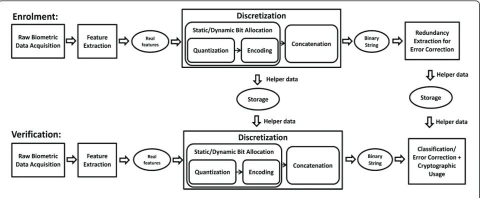
Explosion of biometric-based cryptographic applications (see e.g. [1-12]) in the recent decade has abruptly aug-mented the demand of stable binary strings for identity representation. Biometric features extracted by most current feature extractors, however, do not exist in bin-ary form by nature. In the case where binbin-ary processing is needed,biometric discretizationbecomes necessary in order to transform such an ordered set of continuous features into a binary string. Note that discretization is referred to as a process of‘binarization’ throughout this article. The general block diagram of a biometric discre-tization-based binary string generator is illustrated in Figure 1.
Biometric discretization can be decomposed into two essential components: biometric quantization and fea-ture encoding. These components are governed by a sta-tic or a dynamic bit allocation algorithm, determining whether the quantity of binary bits allocated to every dimension is fixed or optimally different, respectively. Typically, given an ordered set of real-valued feature
elements per identity, each single-dimensional feature space is initially quantized into a number of non-over-lapping intervals according to a quantization fashion. The quantity of these intervals is determined by the cor-responding number of bits assigned by the bit allocation algorithm. Each feature element captured by an interval is then mapped to a short binary string with respect to the label of the corresponding interval. Eventually, the binary output from each dimension is concatenated to form the user’s final bit string.
Apart from the above consideration, information about the constructed feature space for each dimension is stored in the form of helper data to enable reproduc-tion of the same binary string for the same user. How-ever, it is required that such helper data, upon compromise, should neither leak any helpful informa-tion about the output binary string, nor that of the bio-metric feature itself.
In general, there are three aspects that can be used in assessing a biometric discretization scheme:
(1) Performance: Upon extraction of distinctive fea-tures, it is important for a discretization scheme to preserve the significance of real-valued feature ele-ments in the Hamming domain in order to maintain
* Correspondence: [email protected]
School of Electrical and Electronic Engineering, College of Engineering, Yonsei University, Seoul, South Korea
the actual classification performance. A better scheme usually incorporates a feature selection or bit allocation process to ensure only reliable feature components are extracted or highly weighted for obtaining an improved performance.
(2) Security: Helper data upon revelation must not expose any crucial information which may be of assistance to the adversary in obtaining a false accept. Therefore, the binary string of the user should contain adequate entropy and should be completely uncorrelated to the helper data. Gener-ally, entropy is a measure that quantifies the expected value of information contained in a binary string. In the context of biometric discretization, the entropy of a binary string is referred to as the sum of entropy of all single-dimensional binary outputs. With the probabilitypiof every binary outputiÎ {1, ... S} in a dimension, the entropy can be calculated as l=−si=1pilog2pi. As such, the probability pi
will be reduced when the number of outputs S is
increased, signifying higher entropy and security against adversarial brute force attack.
(3) Privacy: A high level of protection needs to be exerted against the adversary who could be inter-ested in all user-specific information other than the verification decision of the system. Apart from the biometric data applicable for discretization, it is important that unnecessary yet sensitive information such as ethnic origin, gender and medical condition should also be protected. Since biometric data is inextricably linked to the user, it can never be reis-sued or replaced once compromised. Therefore, helper data must be uncorrelated to such
information in order to defeat any adversary’s priv-acy violation attempt upon revealing it.
1.1 Related works
Biometric discretization in the literature can generally be divided into two broad categories: supervised and unsupervised discretization (discretization that makes use of class labels of the samples and discretization that does not, respectively).
Unsupervised discretization can be sub-categorized into threshold-based discretization [7-9,11]; equal-width quantization-based discretization [12,13]; and equal-probable quantization-based discretization [5,10,14-16]. For threshold-based discretization, each single-dimen-sional feature space is segmented into two intervals based on a prefixed threshold. Each interval is labeled with a single bit ‘0’or ‘1’. A feature element that falls into an interval will be mapped to the corresponding 1-bit output label. Examples of threshold-based discretiza-tion schemes include Monrose et al.’s [7,8], Teoh et al.’s [9] and Verbitsky et al.’s [11] scheme. However, deter-mining the best threshold could be a hurdle in achieving optimal performance. On top of that, this discretization scheme is only able to produce a 1-bit output per fea-ture dimension. This could practically be insufficient in meeting the current entropy requirement (indicating the level of toughness against brute force attacks).
On the other hand, the unsupervised equal width quantization-based discretization [12,13] partitions each single-dimensional feature space into a number of non-overlapping equal-width intervals during quantization in accordance with the quantity of bits required to be extracted from each dimension. These intervals are labeled with binary reflected gray code (BRGC) [17] for
encoding, where both of which require the number of constructed intervals to be of a power of 2 in order to avoid loss of entropy. Based on the equal-width quanti-zation and the BRGC encoding, Teoh et al. [13] have designed a user-specific equal-width quantization-based dynamic bit allocation algorithm that assigns different number of bits to each dimension based on an intra-class variation measure. Equal width quantization does not incur privacy issue. However, it could not offer maximum entropy since the probability of every quanti-zation output in a dimension is rarely equal. Moreover, the width of quantization intervals can be easily affected by outliers.
The last subcategory of unsupervised biometric discre-tization, known as equal-probable quantization-based discretization [14] segments each single-dimensional fea-ture space into multiple non-overlapping equal-probable intervals, whereby every interval is constructed to encap-sulate an equal portion of background probability mass during quantization. As a result, the constructed inter-vals are of different widths if the background distribu-tion is not uniform. BRGC is used for encoding. Subsequently, two efficient dynamic bit allocation schemes have further been proposed by Chen et al. in [15] and [16] based on equal-probable quantization and BRGC encoding where the detection rate (genuine acceptance rate) [15] as well as area under FRR curve [16] is used as the evaluation measure for bit allocation.
Tuyls et al. [10] and Kevenaar et al. [5] have used a similar equal-probable discretization technique but the bit allocation is limited to at most one bit per dimen-sion. However, a feature selection technique is incorpo-rated in order to identify reliable components based on the training bit statistics [10] or a reliability function [5] so that unreliable dimensions can be eliminated from the overall bit extraction and the discretization perfor-mance can eventually be improved. Equal probable quantization offers maximum entropy. However, infor-mation regarding the background pdf of every dimen-sion needs to be stored so that exact intervals can be constructed during verification. This may pose a privacy threat [18] to the users.
On the other hand, supervised discretization [1,3,14,19] potentially improves classification perfor-mance by exploiting the genuine user’s feature distribu-tion or the user-specific dependencies to extract segmentations which are useful for classification. In Chang et al.’s [1] and Hao-Chan’s scheme [3], single-dimensional interval defined by [μj- ksj, μj+ksj] (also known as thegenuine interval) is first tailored for the Gaussian user pdf (with meanμjand standard deviation sj) of the genuine user with a free parameter k. The remaining intervals of the same width are then con-structed outwards from the genuine interval. Finally, the
boundary intervals are formed by the leftover widths. In fact, the number of bits extractable from each dimen-sion relies on the relative number of formable intervals in that dimension and is controllable byk. This scheme uses direct binary representation (DBR) for encoding. Chen et al. proposed a similar discretization scheme [14] except that BRGC encoding is adopted; the genuine interval is determined by the likelihood ratio pdf; and the remaining intervals are constructed equal-probably. Kumar and Zhang [19] employed an entropy-based quantizer to reduce class impurity/entropy in the inter-vals through recursively splitting every interval until a stopping criterion is met. The final intervals will be resulted in such a way that majority samples enclosed within each interval would belong to a specific identity.
Despite being able to achieve a better classification performance than the unsupervised approaches, a criti-cal problem with these supervised discretization schemes is the potential exposure of the genuine mea-surements or the genuine user pdf, since the con-structed intervals serve as a clue at which the user pdf or measurements could be located to the adversary. As a result, the number of possible locations of user pdf/ genuine measurements might be reduced to the amount of quantization intervals in that dimension, thus poten-tially facilitating malicious privacy violation attempt.
1.2 Motivations and contributions
Past research attention was mostly devoted to proposing discretization schemes with new quantization techniques without realizing the effect of encoding towards the dis-cretization performance. This can be seen from the recent revelation of inappropriateness of DBR and BRGC for feature encoding in classification [20], although they were the most commonly seen encoding schemes for multi-bits discretization in the literature [1,3,12-16]. For this reason, the performance of multi-bits discretization schemes remain to be a mystery when it comes to linking the classification performance in the Hamming domain (discretization performance) with the relative performance in the continuous domain (classifi-cation performance of continuous features). To date, no explicit study has been conducted to resolve such an ambiguity.
an elegant quantization scheme would produce satisfac-tory classification results in the Hamming domain, we adopt the unsupervised equal-width quantization scheme in our analysis due to its simplicity and its less susceptibility against privacy attacks. However, a lower entropy could be achieved when the class distribution is not uniform (with respect to the equal-probable quanti-zation approach). This shortage can simply be tackled by utilizing a larger number of feature dimensions or by allocating a larger quantity of bits to each dimension to compensate such entropy loss.
It is the objective of this article to extend the work of [20] to justify and analyze the deterministic discrete-to-binary mapping behavior of LSSC encoding; as well as
theapproximatecontinuous-to-discrete mapping
beha-vior of equal-width quantization when quantization intervals in each dimension are substantial. We reveal the essential correspondence of distance between the Hamming domain and the rescaled L1 domain for an equal-width quantization and LSSC encoding-based (EW + LSSC) discretization. We further generalize this fundamental correspondence to Lpdistance metrics and inner product-based classifiers to obtain desired perfor-mance resemblances. These important resemblances in fact open up possibility of applying powerful classifier in the Hamming domain such as binary support vector machine (SVM) without having to suffer from a poorer discretization performance with reference to the actual classification performance.
Empirically, we justify the superiority of LSSC over DBR and BRGC and the aforementioned performance resemblances in the Hamming domain by adopting face biometric as our subject of study. Note that such experi-ments could also be conducted using other biometric modalities, as long as the relative biometric features can be represented orderly in the form of a feature vector.
The organization of this paper is described as follows. In the next section, equal-width quantization and LSSC encoding are described as a continuous-to-discrete map-ping and a discrete-to-binary mapmap-ping, respectively, and both mapping functions are derived. These mappings are then combined to reveal the performance resem-blance of EW + LSSC discretization to that of the rescaled L1 distance-based classification. In Section 3, proper methods to extend basic performance resem-blance of EW + LSSC discretization to that of different metrics and classifiers are described. In section 4,
approximateperformance of EW + LSSC discretization
with respect to L1 distance-based classification perfor-mance is experimentally justified. Results showing the resemblances of altered EW + LSSC discretization to the performance of several different distance metrics/ classifier are presented. Finally, several insightful con-cluding remarks are drawn in Section 5.
2. Biometric discretization
For binary extraction, biometric discretization can be described as a two-stage mapping process: Each segmen-ted feature space is first mapped to the respective index of a quantization interval; subsequently, the index of each interval is mapped to a uniquen-bit codeword in a Hamming space. The overall mapping process can be mathematically described by
bdid =g(i
d) =g(f(vd)) (1)
where vd denotes a continuous feature,iddenotes a discrete index of the interval, bdid denotes a short binary
string associated toid, f:ℝ® ℤdenotes a continuous-to-discrete map and g:ℤ® {0, 1}n denotes a discrete-to-binary map. Note that a superscriptdis used for speci-fying the dimension to which a variable belongs and it is by no means of being an integer power. We shall define both these functions in the following subsections.
2.1 Continuous-to-discrete mappingf(·)
A continuous-to-discrete mappingf(·) is achieved through applying quantization to a continuous feature space. Recall that an equal-width quantization divides a one-dimensional feature space evenly in forming the quantization intervals and subsequently maps each interval-captured background probability density func-tion (pdf) to a discrete index. Hence, the probability mass pd
id associated with each indexi
d
precisely repre-sents the probability density captured by the interval with the same index. This equality can be described by
pdid=
intd id(max)
intd id(min)
pdbg(v)dv for id∈ {0, 1, ...,Sd−1} (2)
where pdbg(·) denotes the d-th dimensional back-ground pdf,intd
id(max)andint
d
id(min)denote the upper and
lower boundary of interval with index id in the d-th
dimension, and Sddenotes the number of constructed
intervals in the d-th dimension. Conspicuously, the
resultant background pmf is an approximation of the original pdf upon the mapping.
Suppose that a feature element captured by an interval
intdid with an index i
d
is going to be mapped to a fixed
point within such an interval. Let cdidbe the fixed point
in intd
id to which every feature element v
d
idjd that falls
fromcdidis
εd id,jd=v
d id,jd−C
d
id≤max{int
d id(max)−c
d id,c
d id−int
d id(min)}=ε
d
id,jd(max).(3)
Suppose now we are to match each indexid of theSd intervals with the correspondingcdidthrough some
scal-ing ˆs and translation ˆt:
cdid =ˆsd(id+ˆtd) for id={0,Sd−1}. (4)
To make ˆsd and ˆtd globally derivable for all intervals,
it is necessary to keep distance between cdidand cdid+1 constant for everyid Î{0,Sd- 2}. In order to preserve such a distance between any two different intervals, cdid
in every interval should, therefore, take identical dis-tance from its correspondingintd
id(min). Without loss of
generality, we let cdidbe the central point of intdid, such
that
cdid =
intd
id(max)−intdid(min)
2 for i
d={0,Sd−1}. (5)
With this, the upper bound of distance of vdidjd fromcdid
upon mapping in (3) becomes
εd id,jd≤int
d
id(max)−c
d id =c
d id−int
d
id(min)}=ε
d
id,jd(max). (6)
To obtain the parameters ˆsd and ˆtd, we normalize
both feature and index spaces to (0, 1) and shift every
normalized index id by 1
2Sd to the right to fit the
respectivecdid, such that
cdid
intd
Sd−1 (max)−intd0 (min)
= 2i
d+ 1
2Sd . (7)
Through some algebraic manipulation, we have
cdid =
intd
Sd−1 (max)−intd0 (min)
Sd (i
d+ 0.5). (8)
Thus, ˆsd= int d
Sd−1 (max)−intd0 (min)
Sd and ˆt
d= 0.5.
Combining results from (3), (4) and (8), the continu-ous-to-discrete mapping functionf(·) can be written as
id=f(vdid,jd) = ⎧ ⎪ ⎨ ⎪ ⎩
1
ˆ
sd(v d
id,jd− ˆsdˆt−εidd,jd) for vdid,jd≥cdid
1
ˆ
sd(ˆs dˆt−vd
id,jd−ε
d
id,jd) for v
d id,jd≥c
d id
(9)
Suppose we are to compute a L1 distance between
two arbitrary points vd
id
1,jd1 and vd
id
2,jd2 for all id
1,id2∈[0,Sd−1],jd1,jd2∈ {1, 2...} in the d-th dimen-sional continuous feature space, and the relative distance between the corresponding mapped elements in thed-th dimensional discrete index space, then it is easy to find that the deviation between these two distances can be bounded below:
0≤vdid
2,jd2−v
d id
1,jd1
−cdid
2,jd2−c
d id
1,jd1
≤2εdidjd(max). (10)
From (4), this inequality becomes
0≤vdid
2,jd2− vdid
1,jd1
− ˆs id2−id1≤2εiddjd(max). (11)
Note that the upper bound of such distance deviation is equivalent to the width of an interval in (6), such that
2εdid,jd(max)=intdid(max)−intdid(min). (12)
Therefore, it is clear that an increase or reduction in the width of each equal-width interval could signifi-cantly affect the upper bound of such deviation. For instance, when the number of intervals constructed over a feature space is increased/reduced by a factor ofb(i.e.
Sd® bSdor Sd→ 1
βSd), the width of each equal-width interval will be reduced/increased by the same factor. Hence, the resultant upper bound for the distance
devia-tion becomes2ε
d id,jd(max)
β and 2βε
d
id,jd(max), respectively.
Finally, when static bit allocation is adopted where an equal number of equal-width intervals is constructed in all D feature dimensions, the total distance deviation incurred by the continuous-to-discrete mapping can be upper bounded by 2Dεdid,jd(max).
2.2 Discrete-to-binary mappingg(·)
The discrete-to-binary mapping can be defined in a more direct manner compared to the previous map-ping. Suppose that in the d-th dimension, we have Sd discrete elements to be mapped from the index space. We therefore require the same amount of elements in the Hamming space to be mapped to. In fact, these elements in the Hamming space (also known as the codewords) may have different orders and indices depending on the encoding scheme being employed. With this, the direct-to-binary mapping can, therefore, be specified by
bdid =g(i
d
) = (id) forid∈[0,Sd−1] (13) whereℂ(id) denotes a codeword with index idfrom an
options of ℂand their individual effect on the discrete-to-binary mapping in the following subsections.
2.2.1 Encoding schemes
(a) Direct binary representation (DBR)
In DBR, decimal indices are directly converted into their binary equivalent. Depending on the required size S of a code, the length of DBR is selected to benDBR = [log2 S]. A collection of DBRs in fulfillingS = 4, 8 and 16 are illustrated in Table 1.
(b) Binary reflected gray code (BRGC) [17]
BRGC is a special code that restricts the Hamming distance between every consecutive pair of codewords to unity. Similarly as DBR, each decimal index is uniquely
mapped to one out of S number of nBRGC-bit
code-words, where nBRGC = [log2 S]. If LnBRGC denotes the listing ofnBRGC-bit binary strings, thennBRGC-bit BRGC can be defined recursively as follows:
L1= 0.1
LnBRGC = 0LnBRGC−1,1LnBRGC−1 fornBRGC>1
(14)
Here,bLdenotes the list constructed from Lby add-ing bit bin front of every element of L, and L¯ denotes
the complement of list L. In Table 2, instances of
BRGCs in meeting different values ofSare shown. (c) Linearly separable subcode (LSSC) [20]
Out of 2nL S S C codewords in total for any positive
integer nLSSC, LSSC contains (nLSSC + 1) number of nLS S C-bit codewords, where every adjacent pair of codewords differs by a single bit and every non-adja-cent pair of codewords differs by q bits, withq denot-ing the corresponddenot-ing index difference. Beginndenot-ing with an initial codeword, say the all-zero codeword,
the next nLSSC number of codewords can simply be
constructed by complementing a bit from the lowest order (rightmost) bit position to the highest order (leftmost) bit position one at a time. The resultant nL S S C -bit LSSCs in fulfilling S = 4, 8 and 16 are shown in Table 3.
2.2.2 Mappings and correspondences
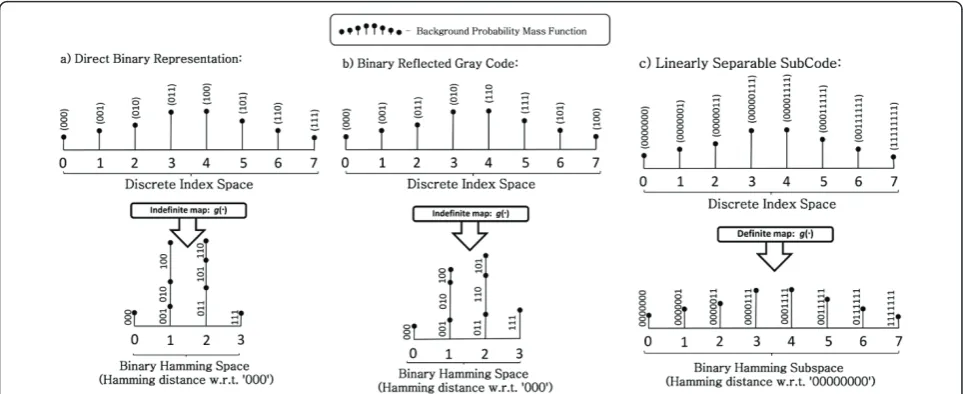
On Hamming space where Hamming distance is crucial, a one-to-one correspondence between each binary code-word and the corresponding Hamming distance incurred with respect to any reference codeword is essentially desired. We can observe clearly from Figure 2 that even though the widely used DBR and BRGC have each of their codewords associated with a unique index, most mapped elements eventually overlap each other as far as Hamming distance is concerned. In other words, although distance deviation in prior continuous-to-discrete mapping is minimal, the deviation effect led by such an overlapping discrete-to-binary mapping could be tremendous, causing the continuous feature elements originated from multiple different non-adjacent intervals to be mapped to a common Hamming distance away from a specific codeword.
Taking DBR as an instance in Figure 2a, feature ele-ments associated with intervals 1, 2 and 4 are mapped to codewords‘001’,‘010’ and‘100’, respectively, which are all 1 Hamming distance away from‘000’(interval 0). This implies that if there is a scenario where we have a genuine template feature captured by interval 0, a genu-ine query feature by interval 1, two imposters’query fea-tures by intervals 2 and 4, all query feafea-tures will be mapped to 1 Hamming distance away from the template
Table 1 A collection ofnDBR-bit DBRs forS= 4, 8 and 16 where [τ] denotes the codeword index
nDBR= 2
S= 4
nDBR= 3
S= 8
nDBR= 4
S= 16
[0] 00 [0] 000 [0] 0000 [8] 1000
[1] 01 [1] 001 [1] 0001 [9] 1001
[2] 10 [2] 010 [2] 0010 [10] 1010
[3] 11 [3] 011 [3] 0011 [11] 1011
[4] 100 [4] 0100 [12] 1100 [5] 101 [5] 0101 [13] 1101 [6] 110 [6] 0110 [14] 1110 [7] 111 [7] 0111 [15] 1111
Table 2 A collection ofnBRGC-bit BRGCs for S = 4, 8 and 16 where [τ] denotes the codeword index
nBRGC= 2
S= 4
nBRGC= 3
S= 8
nBRGC= 4
S= 16
[0] 00 [0] 000 [0] 0000 [8] 1100
[1] 01 [1] 001 [1] 0001 [9] 1101
[2] 11 [2] 011 [2] 0011 [10] 1111
[3] 10 [3] 010 [3] 0010 [11] 1110
[4] 110 [4] 0110 [12] 1010 [5] 111 [5] 0111 [13] 1011 [6] 101 [6] 0101 [14] 1001 [7] 100 [7] 0100 [15] 1000
Table 3 A collection ofnLSSC-bit LSSCs forS= 4,8 and 16 where [τ] denotes the codeword index
nLSSC= 3
S= 4
nLSSC= 7
S= 8
nLSSC= 15
S= 16
and could not be differentiated. Likewise, the same pro-blem occurs when BRGC is employed, as illustrated in Figure 2b. Therefore, these imprecise mappings caused by DBR and BRGC greatly undermine the actual discri-minability of the feature elements and could probably be detrimental to the overall recognition performance.
In contrast, LSSC does not suffer from such a draw-back. As shown in Figure 2c, LSSC links each of its codewords to a unique Hamming distance away from any reference codeword in a decent manner. More pre-cisely, a definite mapping behaviour can be obtained when each index is mapped to a LSSC codeword. The probability mass distribution in the discrete space is completely preserved upon the discrete-to-binary map-ping and thus, a precise mapmap-ping from the L1 distance to the Hamming distance can be expected, such that given two indicesid1=f vdid
1,j
d
1
, id2=f vdid
2,j
d
2
and their
respective LSSC-based binary outputs
id1−id2 =HD bdid
1,b
d id
2
∀id1,id2∈[0,Sd−1],
id1−id2=HD bdid
1 ,bd
id
2
∀id1,id2∈[0,Sd−1] (15)
whereHD denotes the Hamming distance operator.
The only disadvantage of LSSC is the larger bit length requirement a system may need to afford in meeting a similar number of discretization outputs compared to DBR and BRGC. In the case where a total ofSdintervals need to be constructed for each dimension, LSSC intro-ducesRd =Sd- log2 Sd- 1 redundant bits to maintain the optimal one-to-one discrete-to-binary mapping in
the d-th dimension. Thus, upon concatenation of
outputs from all feature dimensions, the length of LSSC-based final binary string could be significantly larger.
2.3 Combinations of both mappings
Through combining both continuous-to-discrete and discrete-to-binary mappings, the overall mapping can be expressed as
bd id
1=g f v
d id
1,jd1
=
⎧ ⎪ ⎪ ⎨ ⎪ ⎪ ⎩ C
1
ˆ
sd v d id,jd− ˆsdˆt−ε
d id,jd
for vd
id,jd≥c
d id
C
1
ˆ
sd ˆs dˆt−vd
id,jd−ε
d id,jd
for vd
id,jd<c
d id
(16)
where ˆsd= int d
Sd−1 (max)−int
d
0 (min)
Sd and ˆt
d= 0.5.
This equation can typically be used to derive the code-word bdid based on the continuous feature value v
d idjd.
In view of different encoding options, three discretiza-tion configuradiscretiza-tions can be deduced. They are:
•Equal Width + Direct Binary Representation (EW
+ DBR)
•Equal Width + Binary Reflected Gray Code (EW +
BRGC)
•Equal Width + Linearly Separable SubCode (EW +
LSSC)
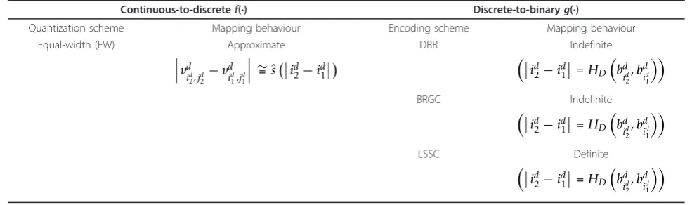
Table 4 gives a glance of the behaviours of both map-pings which we have discussed so far. Among them, a much poorer performance by EW + DBR and EW + BRGC can be anticipated due to intrinsic indefinite mapping deficiency. On contrary, only the combination
of EW + LSSC could lead to approximate and definite
discretization results. Since for LSSC,
HD bdid
2 ,bd
id
1
=id
2−id1 and Sd =ndLSSC+ 1, integrating these LSSC properties with (3) and (4) yield
HD bdid
2,b
d id
1
=id2−id1 = 1
ˆ
sd
cdid
2− cdid
1 = 1 ˆ sd vdid
2,jd2−ε
d id
2,jd2−v
d id
1,jd1+ ε
d id
1,jd1
∼= 1 ˆ
sd
vdid
2,jd2−v
d id
1,jd1
∼= (ndLSSC+ 1) intdSd−1 (max)−int
d
0 (min)
vdid
2,jd2−v
d id
1,jd1
.
(17)
Here the RHS of (17) corresponds to a rescaled L1 distance.
By concatenating distances of all Dindividual dimen-sions, the overall discretization performance of EW + LSSC could, therefore, very likely to resemble the rela-tive performance of the rescaled L1 distance-based clas-sification:
D
d=1
HD bdid
2
,bd id 1 ∼= D d=1 nd
LSSC+ 1 intd
Sd−1 (max)−int
d
0 (min)
vd
id
2,jd2−
vd id
1,jd1
. (18)
Hence, matching plain bitstrings in a biometric verifi-cation system guarantees a rescaled L1 distance-based classification performance when Sd=nd
LSSC+ 1 is ade-quately large. However, for cryptographic key generation applications where a bitstring is derived directly from the helper data of each user for further cryptographic usage, (18) then implies relation between the bit discre-pancy of an identity’s bitstring with reference to the template bitstring and the L1 distance of their continu-ous counterparts in each dimension.
3. Performance resemblances
When binary matching is performed, the basic blance in (18) can further be exploited to obtain resem-blance with the other distance metric-based and machine learning-based classification performance. The key idea for such extension lies in how to flexibly alter the matching function or to represent each continuous feature element individually with its binary approxima-tion in obtaining near-equivalent classificaapproxima-tion behaviour in the continuous domain. As such, rather than just confining binary matching method to pure Hamming distance calculation, these extensions significantly broaden the practicality of performing binary matching and enable a strong performance resemblance of a powerful classifier such as a multilayer perceptron (MLP) [21] or a SVM [22] when the bits allocation to each dimension is substantially large. In this section, ‘ζj’ denotes the matching score of the‘j’ dissimilarity/simi-larity measure.
3.1 LpDistance metrics
In the case where a Lp distance metric classification performance is desired, the resemblance equation in (18) can easily be modified and applied to obtain an approximate performance in the Hamming domain by
ζLp= p
D d=1 vd id
2,jd2−
vd id
1,jd1
p
∼= p
D d=1 ˆ sdid
2−i
d
1
p
∼= p
D d=1 intd
Sd−1 (max)−int d
0 (min)
nd
LSSC+ 1
HD bdid
2,b
d id
1
p
(19)
provided that the number of bits allocated to each dimension are substantially large, or equivalently, the quantization intervals in each dimension are of great
Table 4 A summary of mapping behavior off(·) andg(·)
Continuous-to-discretef(·) Discrete-to-binaryg(·)
Quantization scheme Mapping behaviour Encoding scheme Mapping behaviour Equal-width (EW) Approximate
vd
id
2,jd2− vd
id
1,jd1
∼=ˆsid2−id1
DBR Indefinite
id2−id1 =HD bdid
2,b
d id 1 BRGC Indefinite id
2−id1 =HD bdid
2 ,bd
id
1
LSSC Definite
id
2−id1 =HD bdid
2 ,bd
id
1
number. As long as vdid
2,jd2− vdid
1,jd1
can be linked to the desired distance computation, (14) can then be modified and applied directly. According to (11), the total differ-ence in distance of (19) is upper bounded by
p
D
d=1 2εidd
2,jd2(max)
p
.
Likewise, to achieve a resembled performance of k-NN classifier [23] and RBF network [24] that use Euclidean distance (L2) as the distance metric, the RHS of (19) can simply be amended and subsequently adopted for binary matching by settingp= 2.
3.2 Inner product
For the inner product similarity measure which cannot
be directly associated with vd i2,j2−v
d i1,j1
, the simplest way to obtain the approximate performance resem-blance is to transform each continuous feature value into its binary approximate individually and substitute it into the actual formula. By exploiting results from (3), (8) and (15), we have
vdid,jd∼=
intdSd−1 (max)−int d
0 (min)
nd
LSSC+ 1
(id+ 0.5)
∼=
intd
Sd−1 (max)−int d
0 (min)
nd
LSSC+ 1
(id −0|+ 0.5)
∼=
intd
Sd−1 (max)−int d
0 (min)
nd
LSSC+ 1
HD bdid,b d 0 + 0.5 (20)
leading to an approximate binary representation of the continuous feature value.
Considering inner product (IP) between two column feature vectorsν1 and ν2 as an instance, we represent
every continuous feature element in each feature vector with its binary approximate to obtain an approximately equal similarity measure:
ζIP=vT2v1
= D d=1 vd id 2,jd2
vd id 1,jd1
∼= D d=1 intd
Sd−1 (max)−intd0 (min)
nd
LSSC+ 1
2
id
2+ 0.5
id
1+ 0.5
∼= D d=1 intd
Sd−1 (max)−intd0 (min) nd
LSSC+ 1
2
HD bdid 2
,bd
0
+ 0.5 HD bdid 1
,bd
0
+ 0.5.
(21)
The total similarity deviation of (21) turns out to be
upper bounded byDd=1 εd id,jd(max)
2 .
For another instance, the similarity measure adopted by SVM [22] in classifying an unknown data point appears likewise to be inner product-based. Let nsbe the number of support vectors, yk = ± 1 be the class label of the k-th support vector, vk be the k-th
D-dimensional support (column) vector,vbe the
D-dimen-sional query (column) vector, λˆk be the optimized
Lagrange multiplier of thek-th support vector and wˆo
be the optimized bias. The performance resemblance of binary SVM to that of the continuous counterpart fol-lows directly from (21) in such a way that
ζSVM=
ns
k=1 ykˆλk(vTv
k) +wˆo
=
ns
k=1 ykλˆk
D
d=1 vd
id
2,jd2 vd
id
1,jd1
+wˆo
∼= ns k=1 D d=1 ykˆλk
intd Sd−1 (max)−int
d
0 (min)
nd
LSSC+ 1
2 HD bdid
2
,bd
0
+ 0.5 HD bdid
1
,bd
0
+ 0.5+wˆo.
(22)
The expected upper bound of the total difference in
similarity of (22) is then quantified by
maxyk
nyk
k=1
D
d=1yk εdid
2,jd2(max)
2
where yk = ± 1 and
nyk denotes the number of support vectors with class
labelyk.
In fact, the individual element transformation illu-strated in (20) can be generalized to any other inner product-based measure and classifier such as Pearson correlation [25] and MLP [21] in order to obtain a resemblance in performance when the matching is car-ried out in the Hamming domain.
4. Performance evaluation 4.1 Data sets and experiment settings
To evaluate the discretization performance of the three discretization schemes (EW + DBR, EW + BRGC and EW + LSSC) and to justify the performance resem-blances by EW + LSSC in particular, our experiments were conducted based on the following two popular face data sets:
AR
The employed data set is a random subset of the AR face data set [26], which contains a total of 684 images corre-sponding to 114 identities with 6 images per person. The images were taken under controlled illumination condi-tions with moderate variacondi-tions in facial expressions. The images were aligned according to standard landmarks, such as eyes, nose and mouth. Each extracted raw feature vector consists of 56 × 46 grey pixel elements. Histogram equalization was applied to these images before they were processed by the feature extractor.
FERET
each raw image. The images were pre-processed with histogram equalization before feature extraction. Note that SVM performance resemblance experiments in Fig-ures 3Ib, IIb and 4Ib, IIb only utilize images from the first 75 identities to reduce the computational complex-ity of our experiments.
For each identity in both datasets, half of the images are randomly selected for training while the remaining half is used for testing. In order to measure the false acceptance rate (FAR) of the system, each image of every identity is matched against a random image of every other identity within the testing partition (without overlapping selection), while for evaluating the system FRR, each image is matched against every other images of the same identity for every identity within the testing partition. In the following experiments, the equal error rate (EER) (error rate where FAR = FRR) is used to compare the classification and discretization perfor-mances, since it is a quick and convenient way to
com-pare the accuracy of such classification and
discretization. The lower the EER is, the better the per-formance is considered to be and vice versa.
4.2 Performance assessment
The conducted experiments can be categorized into two parts. The first part examines the performance superior-ity of EW + LSSC over the remaining schemes and jus-tifies the fundamental performance resemblance with the rescaled L1 distance-based classification perfor-mance in (18). The second part vindicates the applic-ability of EW + LSSC discretization in obtaining a resembled performance of each different metric and a classifier including L1, L2, L3 distance metric, inner pro-duct similarity metric and a SVM classifier, as exhibited in (19) and (21). Note that in this part, features from each dimension have been min-max normalized (by
dividing both sides of (19) and (21) by
intd
Sd−1 (max)−intd0 (min)
before they are classified/
discretized.
Both parts of experiments were carried out based on static bit allocation. To ensure consistency of the results, two different dimensionality reduction techniques (prin-cipal component analysis (PCA) [28] and Eigenfeature regularization and extraction (ERE) [29]) with two well-known face data sets (AR and FERET) were used. The raw dimensions of AR (2576) and FERET (4453) images
were both reduced to D= 64 by PCA and ERE in all
parts of experiment.
In general, discretization based on static bit allocation assignsn bits equally to each of theDfeature dimen-sions, thereby yielding a Dn-bit binary string in repre-senting every identity upon concatenating short binary outputs from all individual dimensions. Note that LSSC
has a code length different from DBR and BRGC when labelling a specific number of intervals. Thus, it is unfair to compare the performance of EW + LSSC with the remaining schemes through equalizing the bit length of the binary strings generated by different encoding schemes, since the dimensions utilized by LSSC-based discretization will be much lesser than that by DBR-based and BRGC-DBR-based discretization at common bit lengths.
A better way to compare these discretization schemes would be in terms of entropyLof the final bit string. By denoting the entropy of the d-th dimension asld and the i-th output probability of thed-th dimension as pdid,
we have
L=
D
d=1 ld=−
D
d=1
Sd
i=1
pdidlog2pdid. (23)
Note that due to static bit allocation,Sd =S for all d. SinceSd= 2nfor BRGC & DBR whileS=nLSSC+ 1 for LSSC, Equation 23 becomes
L=
⎧ ⎪ ⎨ ⎪ ⎩
−D
d=1
2n i=1p
d
idlog2pdid for DBR/BRGC encoding based discretization
−D d=1
nLSSC+1
i=1 p
d
idlog2pdid for LSSC encoding based discretization
(24)
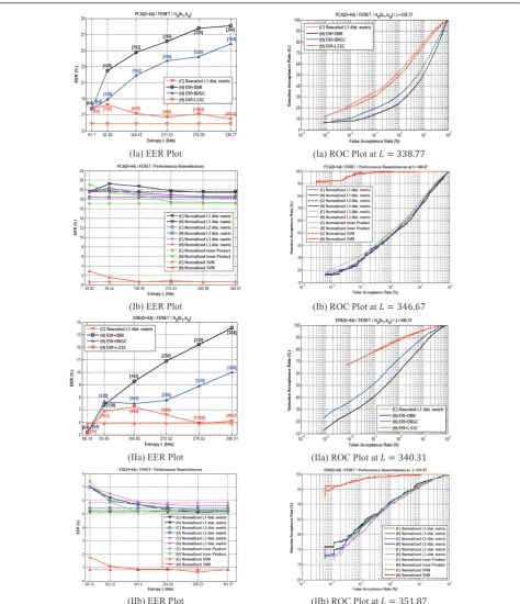
Figure 3 illustrates the EER and the ROC perfor-mances of equal-width based discretization and the per-formance resemblances of EW+LSSC discretization based on the AR face data set. As depicted in Figure 3Ia, IIa for experiments on PCA- and ERE-extracted fea-tures, EW + DBR and EW + BRGC discretizations fail to preserve the distances in the index space and there-fore deteriorate critically as the number of quantization intervals constructed in each dimension increases, or nearly proportionally, as the entropyLincreases. EW + LSSC, on the other hand, achieves not only definite, but also the lowest discretization performance among the discretization schemes especially at high L due to its capability in preserving approximately the rescaled L1 distance-based classification performance.
Another noteworthy observation is that the initially large deviation of EW + LSSC performance from the rescaled L1 distance-based performance tends to decrease as Lincreases at first and fluctuates trivially after a certain point of L. This can be explained by (6) that since for each dimension, the difference between each continuous value with the central point of the interval (to which we have chosen to scale the discreti-zation output) is upper-bounded by half the width of
the interval εd id,jd(max)
. To augment the entropyL
(Ia) EER Plot (Ia) ROC Plot atܮ ൌ ͵ͶͻǤͲ
(Ib) EER Plot (Ib) ROC Plot atܮ ൌ ͵ͶͻǤͲ
(IIa) EER Plot (IIa) ROC Plot atܮ ൌ ͵ͷͳǤʹ
(IIb) EER Plot (IIb) ROC Plot atܮ ൌ ͵ͷͳǤͷͳ
(Ia) EER Plot (Ia) ROC Plot atܮ ൌ ͵͵ͺǤ
(Ib) EER Plot (Ib) ROC Plot atܮ ൌ ͵ͶǤ
(IIa) EER Plot (IIa) ROC Plot atܮ ൌ ͵ͶͲǤ͵ͳ
(IIb) EER Plot (IIb) ROC Plot atܮ ൌ ͵ͷͳǤͺ
the overall deviation 2D εidd,jd(max) can eventually be
obtained. Therefore, the more the number of intervals is constructed for each dimension, or in other words the higher the overall entropy is desired, the stronger the resemblances will be observed to be. Note that similar observations in Figure 3Ia, IIa illustrate the indepen-dence of the resemblances with respect to the feature extraction methods employed.
Perhaps the only limitation arose in achieving such performance resemblances is the inevitable derivation of large length binary string per user when high entropy strength is desired by a system. As shown in Figure 3Ia, IIa, bitstring that is at least four times longer than the entropy is needed to offer 222- and 224-bit entropy respectively, while bit string that is at least six times longer is required to fulfil a 285- and 288-bit system-specific entropy respectively. Indeed, these amounts of binary bits pose high processing challenges to the sys-tem capability. However, with the current state of tech-nology advancement, it is expected that processing these binary strings would not raise so much of a critical threat to the current systems.
For performance resemblance experiments on PCA-and ERE-extracted features in Figure 3Ib, IIb, the ten-dency of the performance resemblances are similar to the previous case where the difference of EER perfor-mance in the continuous and the Hamming domains is
noticeable at low L and an approximate performance
resemblance can be noticed when L≥ 159.2 in Figure
3Ib and L ≥ 161.7 in Figure 3IIb. Therefore, similar
explanations applied.
Similar performance trends can be seen in Figure 4
when FERET data set was used. Note that when L
increases, EW + DBR and EW + BRGC remain deterior-ating badly, as shown in Figure 4Ia, IIa. Their deficit of being indefinite during the discrete-to-binary mapping process can again be justified. Contrarily, the perfor-mance of the EW + LSSC discretization remains the lowest and it resembles nearly exactly the rescaled L1
distance-based performance whenL≥ 338.77 in Figure
4Ia and L≥276.52 in Figure 4IIa. In Figure 4Ib, IIb, the initial performance deviation between each pair of schemes is slightly lower as those in Figure 4Ib, IIb, although perfect resemblance can similarly be observed at highL.
4.3 Summary and discussions
By and large, our general findings can be summarized in the following three aspects:
• When substantial quantization intervals are
con-structed or a large number of bits are allocated to each feature dimension, equal width (EW) quantization offers an approximate continuous-to-discrete mapping. LSSC
outperforms DBR and BRGC in preserving a definite discrete-to-binary mapping behaviour. Overall, adopting equal width quantization with LSSC as a discretizer results in an approximate outcome.
• As long as EW+LSSC is concerned, the distance
between two mapped elements in the Hamming domain is fundamentally associated to an approximately rescaled L1 distance between the two continuous counterparts.
•The basic performance resemblance of EW + LSSC
discretization to L1 distance-based classification can be extended to Lpdistance-based and inner product-based classifications either by flexibly modifying the matching function or by substituting every continuous feature ele-ment individually with its binary approximate to obtain a similar classification behaviour in the continuous domain.
We believe that the clarification of the underlying mapping behaviours of EW + LSSC discretization would benefit not only the cryptographic and biometric com-munities, but also communities from machine learning and data mining areas (i.e. relevant applications include image retrieval [30], image categorization [31], text cate-gorization [32] and etc). In fact, EW + LSSC discretiza-tion can be appropriately adopted in any other application that requires transformation from continu-ous data to binary bitsrings and involves similarity/dis-similarity matching in the Hamming domain so as to attain a deterministically resembled performance of the continuous counterpart.
5. Conclusion
These analysis outcomes have been experimentally sup-ported and the performance resemblances which we have shown are neither dependent to the feature extrac-tion technique (PCA and ERE) nor the dataset (AR and FERET).
List of abbreviations
BRGC: binary reflected gray code; DBR: direct binary representation; EER: equal error rate; ERE: Eigenfeature regularization and extraction; EW: equal width; FAR: false acceptance rate; IP: inner product; LSSC: linearly separable subcode; MLP: multilayer perceptron; PCA: principal component analysis; SVM: support vector machine.
Acknowledgements
This work was supported by the MKE (The Ministry of Knowledge Economy), Korea, under IT/SW Creative research program supervised by the NIPA (National IT Industry Promotion Agency) (NIPA-2010-(C1810-1002-0016)).
Competing interests
The authors declare that they have no competing interests.
Received: 31 January 2011 Accepted: 10 October 2011 Published: 10 October 2011
References
1. Y Chang, W Zhang, T Chen, Biometric-based cryptographic key generation, inProceedings of IEEE International Conference on Multimedia and Expo (ICME 2004), (2004)
2. Y Dodis, R Ostrovsky, L Reyzin, A Smith, Fuzzy extractors: How to generate strong keys from biometrics and other noisy data. inEurocrypt 2004, LNCS. 3027, 523–540 (2004). doi:10.1007/978-3-540-24676-3_31
3. F Hao, CW Chan, Private key generation from on-line handwritten signatures. Inf Manage Comp Security10(4), 159–164 (2002). doi:10.1108/ 09685220210436949
4. A Juels, M Wattenberg, A fuzzy commitment scheme, in6th ACM Conference in Computer and Communication Security (CCS’99), 28–36 (1999) 5. TAM Kevenaar, GJ Schrijen, M van der Veen, AHM Akkermans, F Zuo, Face
recognition with renewable and privacy preserving binary templates, in Proceedings of 4th IEEE Workshop on Automatic Identification Advanced Technologies (AutoID‘05), 21–26 (2005)
6. J-P Linnartz, P Tuyls, New shielding functions to enhance privacy and prevent misuse of biometric templates, inProceedings of 4th International Conference on Audio and Video Based Person Authentication (AVBPA 2004), LNCS.2688, 238–250 (2003)
7. F Monrose, MK Reiter, Q Li, S Wetzel, Cryptographic key generation from voice, inProceedings of IEEE Symposium on Security and Privacy (S&P 2001), 202–213 (2001)
8. F Monrose, MK Reiter, Q Li, S Wetzel, Using voice to generate cryptographic keys, inProceedings of Odyssey 2001, The Speaker Verification Workshop (2001)
9. ABJ Teoh, DCL Ngo, A Goh, Personalised cryptographic key generation based on FaceHashing. Comput. Security23(7), 606–614 (2004). doi:10.1016/ j.cose.2004.06.002
10. P Tuyls, AHM Akkermans, TAM Kevenaar, G-J Schrijen, AM Bazen, NJ Veldhuis, Practical biometric authentication with template protection, in Proceedings of 5th International Conference on Audio- and Video-based Biometric Person Authentication, LNCS.3546, 436–446 (2005). doi:10.1007/ 11527923_45
11. E Verbitskiy, P Tuyls, D Denteneer, JP Linnartz, Reliable biometric authentication with privacy protection, in24th Benelux Symposium on Information Theory, 125–132 (2003)
12. WK Yip, Goh A, Ngo DCL, Teoh ABJ, Generation of replaceable
cryptographic keys from dynamic handwritten signatures, inProceedings of 1st International Conference on Biometrics, Lecture Notes in Computer Science. 3832, 509–515 (2006)
13. ABJ Teoh, WK Yip, K-A Toh, Cancellable biometrics and user-dependent multi-state discretization in BioHash. Pattern Anal Appl.13(3), 301–307 (2009)
14. C Chen, R Veldhuis, T Kevenaar, A Akkermans, Multi-bits biometric string generation based on the likelihood ratio, inProceedings of IEEE International Conference on Multimedia and Expo (ICME 2004).3, 2203–2206 (2004) 15. C Chen, R Veldhuis, T Kevenaar, A Akkermans, Biometric quantization through detection rate optimized bit allocation. EURASIP J Adv Signal Process.16(2009)
16. C Chen, R Veldhuis, Extracting biometric binary strings with minimal area under the FRR curve for the Hamming distance classifier. Signal Process.91, 906–918 (2011). doi:10.1016/j.sigpro.2010.09.008
17. F Gray, Pulse code communications. U.S Patent.2632058(1953)
18. J Galbally, J Fierrez, J Ortega-Garcia, C McCool, S Marcel, Hill-climbing attack to an Eigenface-Based face verification system, in1st IEEE International Conference on Biometrics, Identity and Security (BIdS), 1–6 (2009) 19. A Kumar, D Zhang, Hand geometry recognition using entropy-based
discretization. IEEE Trans Inf Forens Security, 2, 181–187 (2007)
20. M-H Lim, ABJ Teoh, Linearly separable subcode, A novel output label with high separability for biometric discretization, inProceedings of 5th IEEE Conference on Industrial Electronics and Applications (ICIEA’10)(2010) 21. H Simon,Neural Networks: A Comprehensive Foundation, Second Edition
(Prentice Hall, New York, 1998)
22. C Cortes, V Vapnik, Support-vector networks. Mach Learn.20(3), 273–297 (1995)
23. TM Cover, PE Hart, Nearest neighbor pattern classification. IEEE Trans Inform Theory13(1), 21–27 (1967)
24. MD Buhmann,Radial Basis Functions: Theory and Implementations (Cambridge University, Cambridge, United Kingdom, 2003)
25. K Pearson, Notes on the history of correlation. Biometrika13(1), 25–45 (1895)
26. AM Martinez, R Benavente, The AR Face Database. CVC Technical Report # 24 (1998)
27. PJ Philips, H Moon, PJ Rauss, S Rizvi, The FERET evaluation methodology for face recognition algorithms. IEEE Trans Pattern Anal Mach Intell.22(10) (2000)
28. M Turk, A Pentland, Eigenfaces for recognition. J Cognit, Neurosci.3(1), 71–86 (1991). doi:10.1162/jocn.1991.3.1.71
29. XD Jiang, B Mandal, A Kot, Eigenfeature regularization and extraction in face recognition. IEEE Trans Pattern Anal Mach Intell.30(3), 383–394 (2008) 30. R Datta, D Joshi, J Li, JZ Wang, Image retrieval: ideas, influences, and trends
of the new age. ACM Comput Surveys40(2), 1–60 (2008)
31. Y Chen, JZ Wang, Image categorization by learning and reasoning with regions. J Mach Learn Res.5, 913–939 (2004)
32. F Sebastiani, Machine learning in automated text categorization. ACM Comput Surveys34(1), 1–47 (2002). doi:10.1145/505282.505283
doi:10.1186/1687-6180-2011-82
Cite this article as:Limet al.:An analysis on equal width quantization and linearly separable subcode encoding-based discretization and its performance resemblances.EURASIP Journal on Advances in Signal Processing20112011:82.
Submit your manuscript to a
journal and benefi t from:
7Convenient online submission
7Rigorous peer review
7Immediate publication on acceptance
7Open access: articles freely available online
7High visibility within the fi eld
7Retaining the copyright to your article
![Table 2 A collection of n16 where [BRGC-bit BRGCs for S = 4, 8 andτ] denotes the codeword index](https://thumb-us.123doks.com/thumbv2/123dok_us/1146111.1143828/6.595.307.538.603.730/table-collection-brgc-brgcs-andt-denotes-codeword-index.webp)