Multivariate spatial nonparametric modelling
via kernel processes mixing
∗
Montserrat Fuentes and Brian Reich
SUMMARY
In this paper we develop a nonparametric multivariate spatial model that avoids specifying
a Gaussian distribution for spatial random effects. Our nonparametric model extends the
stick-breaking (SB) prior of Sethuraman (1994), which is frequently used in Bayesian
mod-elling to capture uncertainty in the parametric form of an outcome. The stick-breaking prior
is extended here to the spatial setting by assigning each location a different, unknown
dis-tribution, and smoothing the distributions in space with a series of space-dependent kernel
functions that have a space-varying bandwidth parameter. This results in a flexible
nonsta-tionary spatial model, as different kernel functions lead to different relationships between the
∗M. Fuentes is a Professor of Statistics at North Carolina State University (NCSU). Tel.: (919) 515-1921,
Fax: (919) 515-1169, E-mail: [email protected]. B. Reich is an Assistant Professor of Statistics at
NCSU. The authors thank the National Science Foundation (Reich, DMS-0354189; Fuentes DMS-0706731,
DMS-0353029), the Environmental Protection Agency (Fuentes, R833863), and National Institutes of Health
(Fuentes, 5R01ES014843-02) for partial support of this work. Key words: dirichlet processes,
distributions at nearby locations. This approach is the first to allow both the probabilities
and the locations of the SB prior to depend on space, and that way there is no need for
replications and we obtain a continuous process in the limit. We extend the model to the
multivariate setting by having for each process a different kernel function, but sharing the
location of the kernel knots across the different processes. The resulting covariance for the
multivariate process is in general nonstationary and nonseparable. The modelling framework
proposed here is also computationally efficient because it avoids inverting large matrices and
calculating determinants, which often hinders the spatial analysis of large data sets. We
study the theoretical properties of the proposed multivariate spatial process. The methods
are illustrated using simulated examples and an air pollution application to model speciated
particulate matter.
1
Introduction
This paper focuses on the problem of modelling the unknown distribution of a multivariate
spatial process. We introduce a nonparametric model that avoids specifying a Gaussian
distribution for the spatial random effects, and it is flexible enough to characterize the
po-tentially complex spatial structures of the tail and extremes of the multivariate distribution.
We develop a new multivariate model that overcomes the assumption of normality,
stationarity and/or separability, and is computationally efficient. The assumption of
sep-arability offers a simplified representation of any variance-covariance matrix, and
conse-quently, some remarkable computational benefits. The concept of separability refers a
co-variance matrices, for example a multivariate spatial coco-variance is often modeled as the
kronecker product of a spatial covariance matrix and a cross-covariance matrix. Suppose
that {Y(s) : s ≡ (s1, s2,· · · , sd)′ ∈ D ⊂ Rd} denotes a spatial process where s is a
spa-tial location over a fixed domain D, Rd is a d-dimensional Euclidean space. The spatial
covariance function is defined as C(si −sj) ≡ cov{Y(si), Y(sj)}, where si = (si1,· · · , sid)′
and C is positive definite. Under the assumption of stationarity, we haveC(si−sj)≡C(h),
whereh≡(h1,· · · , hd)′ =si−sj. However, in real applications, especially with air pollution
data, it may not be reasonable to assume that the covariance function is stationary. Spatial
models often assume the outcomes follow normal distributions, or that the observations are
a realization of a Gaussian process. However, the Gaussian assumption is overly restrictive
for pollution data, which often display heavy tails that change across space. We propose
here a new nonparametric (Dirichlet-type) multivariate spatial model flexible enough to
characterize extreme events in the presence of complex spatial structures, that allows for
nonstationarity in both the covariance and cross-covariance between outcomes.
Our nonparametric model extends the stick-breaking (SB) prior of Sethuraman (1994),
which is frequently used in Bayesian modelling to capture uncertainty in the parametric
form of an outcome’s distribution. The SB prior is a special case of the priors neutral to the
right (Doksum, 1974). For general (non-spatial) Bayesian modelling, the stick-breaking prior
offers a way to model a distribution of a parameter as an unknown quantity to be estimated
from the data. The stick-breaking prior for the unknown distribution F, is
F =d
M
X
i=1
piδ(Xi),
Beta(ai, bi) independent across i, δ(Xi) is the Dirac distribution with point mass at Xi,
Xi iid
∼ Fo, andFo is a known distribution. A special case of this prior is the Dirichlet process
prior with infinite M and Vi iid
∼ Beta(1, ν) (Ferguson, 1973). The stick-breaking prior has
been extended to the univariate spatial setting by incorporating spatial information into the
either the model for the locationsXi or the model for the massespi. Gelfand et al. (2005a),
Gelfand, Guindani and Petrone (2007), and Petrone, Guindani and Gelfand (2008) model
the locations as vectors drawn from a spatial distribution, in particular Petrone, Guindani
and Gelfand (2008) extend this type of Dirichlet mixture model for functional data analysis.
However, their model requires replication. Griffin and Steel (2006) propose a spatial Dirichlet
model that permutes the Vi based on spatial location, allowing the occurrence of Xi to be
more or less likely in different regions of the spatial domain. Reich and Fuentes (2007)
introduce a SB prior allowing the probabilities pi to be space-dependent, by using kernel
functions that have independent and identically distributed (iid) bandwidths, this spatial
SB prior has a limiting process that is not continuous. This model is similar to that of
Dunson and Park (2008), who use kernels to smooth the weights in the non-spatial setting.
An et al. (2008) extend the kernel SB prior for use in image segmentation. Reich and
Fuentes (2007) use the kernel SB prior in a multivariate setting, but it has a separable
cross-covariance.
Here we introduce for the first time an extension of the stick-breaking prior to the
mul-tivariate spatial setting allowing for nonseparability in the spatial cross-dependency between
the outcomes of interest. The stick-breaking prior is extended here to the spatial setting by
assigning each location a different, unknown distribution, and smoothing the distributions
band-width parameter. This results in a flexible nonstationary spatial model, as different kernel
functions lead to different relationships between the distributions at nearby locations. This
approach we introduce here is the first to allow both the probabilitiespi and the locationsXi
to depend on space, and that way there is no need for replications and we obtain a continuous
process in the limit. We extend the model to the multivariate setting, by using a multivariate
version of the space-dependent kernel SB prior, having for each process a different kernel
function, but sharing the location of the kernel knots across the different processes. The
resulting marginal covariance for the multivariate process is in general nonstationary and
nonseparable.
One of the main challenges when analyzing continuous spatial processes and making
Bayesian spatial inference is calculating the likelihood function of the covariance parameters.
For large datasets, calculating the determinants that we have in the likelihood function might
not be feasible. The modelling framework proposed here is computationally efficient because
it avoids inverting large matrices and calculating determinants.
The application presented in this paper is in air pollution, to model and characterize
the complex spatial structure of speciated fine particulate matter. Fine particulate matter
(PM2.5) is an atmospheric pollutant that has been linked to serious health problems,
in-cluding mortality. The study of the association between ambient particulate matter (PM)
and human health has received much attention in epidemiological studies over the past few
years. ¨Ozkaynak and Thurston (1987) conducted an analysis of the association between
several particle measures and mortality. Their results showed the importance of considering
particle size, composition, and source information when modeling particle pollution health
total carbonaceous mass, ammonium, and crustal material. These components have
com-plex spatial dependency and cross dependency structures. The PM2.5 chemistry changes
with space and time so its association with mortality could change across space and time.
Dominici et al. (2002) showed that different cities have different relative risk of mortality
due to PM2.5 exposure. It is important to gain insight and better understanding about the
spatial distribution of each component of the total PM2.5 mass, and also to estimate how the
composition of PM2.5 might change across space. This type of analysis is needed to conduct
epidemiological studies of the association of these pollutants and adverse health effects. We
introduce a innovative multivariate spatial model for speciated PM2.5across the entire United
States. The proposed framework captures the cross dependency structure among the PM2.5
components and explains their spatial dependency structures. Due to the complex
cross-dependency between PM2.5 components, it is important to introduce a statistical framework
flexible enough to allow the cross-dependency between pollutants to be space-dependent,
while allowing for nonstationarities in the spatial structure of each component. This is the
first study with speciated particulate matter that allows the cross-dependency between
com-ponents vary spatially. In the context of air pollution we are interested in extreme values
(hot spots), so we need spatial models that go beyond the assumption of normality. The
multivariate spatial SB model introduced in this paper seems to provide an ideal framework
to characterize the complex structure of the speciated PM2.5.
The paper is organized as follows. In Section 2, we introduce a new spatial univariate
spatial model using an extension of the stick-breaking prior, that directly models
nonstation-arity. In Section 3, we present a multivariate extension of this spatial SB model, that allows
In Section 4, we introduce a particular case of the multivariate spatial model presented in
Section 3, which is a simple model and very easy to implement, but general and flexible
enough for many applications. In Section 5, we present the conditional properties of the
spatial SB process prior. In Section 6, we present marginal properties. In Section 7, we
study some asymptotic properties of the spatial SB prior. In Section 8, we present and
prove an important feature of our model, which is that the limiting process has continuous
realizations. In Section 9, we include some computational approaches and Markov Chain
Monte Carlo(MCMC) details for its implementation. In Section 10, we illustrate the
pro-posed methods with a simulation study. In Section 11, we present an application to air
pollution. We conclude with Section 12 that has some remarks and final comments.
2
Univariate spatial model
The spatial distribution of a stochastic process Y(s) is modeled using an extension of the
stick-breaking prior, that directly models nonstationarity. The nonparametric spatial model
assigns a different prior distribution to the stochastic process at each location, i.e., Y(s)∼
Fs(Y). The distributions Fs(Y) are unknown and smoothed spatially. The coordinate s is
in D ∈ Rd, in particular for d = 3 this could correspond to a continuous spatial temporal
process. To simplify notation throughout this section we will assume d= 2.
Extending the stick-breaking prior to depend on location, the prior for Fs(Y) is the
potentially infinite mixture
Fs(Y)= M
X
i=1
pi(s)δ(X(φi)) = M
X
i=1
Vi(s)
Y
j<i
[1−Vj(s)]δ(X(φi)), (1)
V1(s), pi(s) = Vi(s)Qij−=11(1−Vj(s)), and Vi(s) = Ki(s)Vi, Vi ∼Beta(a, b) independent over
i. The weight function, Ki, is a spatial kernel centered at φi with bandwidth parameter ǫi.
More generally, in our application we fit elliptical kernelsKi, withBi being the 2×2 matrix
that controls the ellipse. We representBi =T(φi)T(φi)′,whereT(φi)′ denotes the transpose
of T(φi), and Tkk′(φi) is the (k, k′) element of the matrix T(φi), log(T11(φi)), log(T22(φi)),
and T12(φi) are independent spatial Gaussian processes.
As we will see in Sections 5 and 6 the spatial correlation of the processY(s) is controlled
by the bandwidth parameters associated with knots in the vicinity of s. To allow the
corre-lation to vary from region to region, the bandwidth parameters are modeled as a spatially
varying parameters. We assign to log(T(φi)) a spatial Gaussian prior with non-zero mean
and a Mat´ern correlation function (Mat´ern, 1960). We assume the Mat´ern spatial correlation
with the parameterization proposed by Handcock and Wallis (1994), that is,
corr(log(T(φi)),log(T(φj)) =
(2ν1/2|φ
i−φj|/ρ)ν
2ν−1Γ(ν) Kν(2ν 1/2|φ
i−φj|/ρ),
whereKνis the modified Bessel function, and|φi−φj|denotes the Euclidean distance between
φi and φj. The Mat´ern correlation has two parameters: ν controls the smoothness of the
process (i.e., the degree of differentiability), and ρ controls the range of spatial correlation.
If ν = 0.5 we have the exponential correlation exp(|φi−φj|/ρ), and if ν = ∞ we have the
squared-exponential correlation exp(|φi−φj|2/ρ2).
In addition to allowing the correlation (via the bandwidth parameters) to be a function
of space, we also allow the variance to be a spatial process. To do this, the spatial process
X(φi) has a zero mean-Gaussian process prior with covariance (Palacios and Steel, 2006),
where σi =σ(φi) is the the variance of the process X(φi) and it is space-dependent, and ρ
is a correlation function (e.g. a Mat´ern). We assign to log(σ(φi)) a spatial Gaussian prior,
with non-zero mean and a Mat´ern covariance function.
In Appendix A.1 we prove that the representation in (1) introduces a properly defined
process prior, using the Kolmogorov existence theorem. In Sections 6 and 7 we study the
marginal and conditional properties of model (1). If the knots are uniformly distributed
across space, the bandwidth parameters are not space-dependent functions, σi =σ for all i,
and the prior distributions for the knots, bandwidth parameters and Vi’s are independent,
then, the corresponding covariance (integrating out Vi, φi, T) assuming the kernel is not
space-dependent, i.e. is stationary (as shown in Section 7). Allowing the bandwidth to be
space-dependent will make it nonstationary (Section 7). The conditional covariance will be
in general nonstationary, even when the kernels are not space-dependent (Section 6).
Model (1) is a Dirichlet Process (DP) mixture model with spatially varying weights.
The almost sure discreteness of Fs(Y) is not desirable in practice. Thus, we mix it with a
pure error process (nugget process) with respect to Fs(Y) to create a random distribution
process Gs(Z) with continuous support (Gelfand et al., 2005). Thus, the process of interest
that we model in practice is Z(s) =Y(s) +e(s),where Y arrives from the DP model in (1),
and e(s) ∼N(0, σ2
0). We denote Σe the diagonal covariance of the nugget process e. Thus,
3
Multivariate spatial model
We present a new nonparametric multivariate spatial model, which is a multivariate extension
of model (1). We explain the cross spatial dependency between p stochastic processes,
Y1(s), . . . , Yp(s), by introducing the following model for the distribution of eachYk(s),
Fs(Yk) = M
X
i=1
Vi,k(s)
Y
j<i
[1−Vj,k(s)]δ(Xk(φi)), (3)
where, p1,k(s) = V1,k(s), pi,k(s) = Vi,k(s)Qij−=11(1−Vj,k(s)), and Vi,k(s) = Ki,k(s)Vi, Vi ∼
Beta(a, b) independent over i, the knots of the kernel functions Ki,k are shared across the
p space-time processes, and the p-dimensional process X = (X1, . . . , Xp) has a multivariate
normal prior, with cross covariance
cov((X1(φ1), . . . , Xp(φ1)),(X1(φ2), . . . , Xp(φ2))) =C(φ1, φ2) =
k
X
j=1
ρj(φ1−φ2)gj(φ1)gjt(φ2)
(4)
with gj the jth column of a p×p full rank matrix G, and the ρj are correlation functions
(e.g., Mat´ern functions). Equation (4) presents a nonstationary extension of a linear model
of coregionalization (Gelfand et al, 2004). Gelfand et al. (2004) characterize the
cross-covariance of a multivariate Gaussian process X using a spatial Wishart prior. Here, we
propose an alternative framework, that could be more computationally efficient.
The cross-covariance for the multivariate processX at each knotiis Σ(i) =A(φ
i)A′(φi),
where A is a full rank lower triangular, A(φi) = {akk′(φi)}kk′, and for each k and k′ in
{1, . . . , p}, akk′ are independent spatial Gaussian non-zero mean processes evaluated at
lo-cation φi. For identification purposes we restrict the mean of the diagonal elements of A
to be positive. Thus, the process (X1(φi), . . . , Xp(φi)) has a multivariate normal prior with
i, and therefore change with location, we obtain a cross covariance between the Yk processes
that varies with space (nonstationarity), and it is in general nonseparable, in the sense that
we do not model separately the cross-dependency between the p processes and the spatial
dependency structure. We allow not only the magnitude of the cross-dependency structure
to vary across space but also its sign, thus, it could be negative in some areas and positive
in others. We call this phenomenon “nonstationarity for the sign” of the cross-dependency.
Most multivariate models, in particular separable models for the covariance, constrain the
cross-dependency to be stationary with respect to its sign (e.g., Reich and Fuentes, 2007;
Choi, Reich, Fuentes, and Davis, 2008).
4
Particular case
A simpler representation of the nonparametric multivariate spatial model in (3), would be
obtained by sharing the univariate underlying process X across thep spatial processes, i.e.
having the following representation for the distribution of each Yk(s),
Fs(Yk) = M
X
i=1
Ki,k(s)Vi,k
Y
j<i
[1−Kj,k(s)Vj,k]δ(X(φi)),
where theV andK random weights are different for each process Yk. This allows the spatial
processesYk,withk = 1, . . . , p,to have different spatial structure. TheV andK components
explain the different spatial structure of theYk processes, as well as the strength of the
cross-dependence between the Y′
ks. This simpler version can offer computational benefits but it
5
Conditional properties
5.1
Conditional univariate spatial covariance
Assume the spatial stick-breaking process priorFs(Y) in (1) for the data processY.
Through-out this section, withThrough-out loss of generality, we assume Bi =ǫiI, where I is the 2×2 identity
matrix. Conditional on the probability masses pi(s) in (1) but not on the latent processX,
the covariance between two observations is as follows,
cov(Y(s), Y(s′)|p(s), p(s′), C) = X
i
σ2ipi(s)pi(s′) +
X
i16=i2
pi1(s)pi2(s ′)C(|φ
i1 −φi2|)
= X
i
σ2i
"
Ki(s)Ki(s′)Vi2
Y
j<i
(1−((Kj(s) +Kj(s′))Vj +Kj(s)Kj(s′)Vj2))
#
+ X
i16=i2
[Ki1(s)Ki2(s ′
)Vi1Vi2C(φi1 −φi2)
Y
j1<i1 Y
j2<i2
(1−(Kj1(s)Vj1 +Kj2(s ′
)Vj2) +Kj1(s)Kj2(s ′
)Vj1Vj2)], (5)
where p(s) = (p1(s), p2(s), . . .) denotes the potentially infinite dimensional vector with all
the probability massespi(s) in the mixture presented in (1), C is the covariance function of
X, and σ2
i = cov(X(φi), X(φi)).
The conditional covariance of the data process Y in (5) between any two locationss and
s′ is stationary and approximates the covariance function C of the underlying process X,
cov(X(s), X(s′)) = C(|s−s′|), as the bandwidths of the kernel functions become smaller.
This interesting result is formally presented in Theorem 1.
Theorem 1.
Assuming the spatial stick-breaking process prior Fs(Y) presented in (1) for a data
The conditional covariance of the data process Y between any two locations s and s′,
cov(Y(s), Y(s′)), approximates the covariance function C of the underlying processX,
eval-uated at |s −s′|, as the bandwidth parameter ǫ
i of each kernel function Ki in (1) goes
uniformly to zero for alli, i.e. ǫi < ǫ, for alli, such thatǫ→0. Assuming thatKi is a kernel
with compact support for alli, and thatC has a first order derivative, C′, that is a bounded
nonnegative function.
Proof of Theorem 1: In Appendix A.2.
5.2
Conditional multivariate spatial covariance
Assuming the multivariate spatial stick-breaking process prior (Fs(Y1), . . . , Fs(Yp)) in (3) for
the data processes Y1(s), . . . , Yp(s), and conditioning on the probabilities pi,1(s) and pi,2(s′)
for each pair of data processes Y1(s) and Y2(s′), but not on the corresponding underlying
multivariate processX = (X1, X2). Then, the conditional cross-covariance between any pair
Y1(s) and Y2(s2),is
cov(Y1(s), Y2(s′)|p1(s), p2(s′), C) =
X
i
pi,1(s)pi,2(s′)C1,2(φi, φi)
+ X
i16=i2
pi1,1(s)pi2,2(s ′
)C1,2(φi1, φi2)
= X
i
[Ki,1(s)Ki,2(s′)Vi,1Vi,2C1,2(φi, φi)
Y
j<i
(1−Kj,1(s)Vj,1−Kj,2(s′)Vj,2+Kj,1(s)Kj,2(s′)Vj,1Vj,2)]
+ X
i16=i2
[Ki1,1(s)Ki2,2(s ′)V
i1,1Vi2,2C1,2(φi1, φi2)
Y
j1<i1 Y
j2<i2
(1−(Kj1,1(s)Vj1,1+Kj2,2(s ′
)Vj2,2) +Kj1,1(s)Kj2,2(s ′
)Vj1,1Vj2,2) #
. (6)
approximates the cross-covariance function cov(X1(s), X2(s′)) = C1,2(s, s′) of the underlying
process X = (X1, X2) used to defined the process prior for Y1 and Y2, as the bandwidth
parameters of the kernel functions become smaller. This result is formally presented in
Theorem 2.
Theorem 2.
Assuming the multivariate spatial stick-breaking process prior (Fs(Y1), . . . , Fs(Yp)) in
(3) for the data processes Y1(s), . . . , Yp(s), and conditioning on the probabilities pi,1(s) and
pi,2(s′) for each pair of data processes Y1(s) and Y2(s′), but not on the corresponding
un-derlying multivariate process X = (X1, X2). Assuming also that C1,2, the cross-covariance
function cov(X1(s), X2(s′)) = C1,2(s, s′) of the underlying process X = (X1, X2), has first
order partial derivatives that are bounded nonnegative functions, and the kernels functions
used in the definition of the probabilities pi,1(s), pi,2(s′) for each data process Y1(s) and
Y2(s) have compact support. Then, the conditional cross-covariance between any pair Y1(s)
and Y2(s2), cov(Y1(s), Y2(s′)), approximates the cross-covariance function C1,2(s, s′) of the
underlying process X, as the bandwidth parameters ǫi,1 and ǫi,2 of the kernel functions in
Fs(Y1) and Fs(Y1) go uniformly to zero for all i, i.e. ǫi,k < ǫ, for all i and for k = 1,2, with
ǫ→0.
6
Marginal properties
6.1
Univariate
We study the marginal properties of the spatial stick prior representation in (1). We start
assuming that the Vi components in (1) are independent and they share the same prior
Vi ∼ Beta(a, b). Then, E(Vi) = E(V), and E(Vi2) = E(V2), for all i. Throughout this
section, without loss of generality, we assumeBi =ǫiI, whereI is the 2×2 identity matrix.
We also assume the covariance, C, of the underlying process X is a stationary covariance,
such that C(0) = σ2, and it is also an integrable function. We consider independent priors
for the bandwidth and the knot parameters of the kernel functions Ki. In the following
section we will study the marginal properties when the Vi components are space dependent
functions and X has a nonstationary variance.
Integrating over the probability masses, the marginal covariance between two
observa-tions is
cov(Y(s), Y(s′))
= σ2c
2E(V2)
X
i
1−2c1E(V) +c2E(V2)
i−1
+ X
i16=i2
c1,2[1−2c1E(V) +c2E(V)2](i1−1)(i2−1)
= σ2 γ(s, s
′)
2(1 +b/(a+ 1))−γ(s, s′)+E(V)
2 X
i16=i2
where
γ(s, s′) = R R
Ki(s)Ki(s′)p(φi, ǫi)dφidǫi
R R
Ki(s)p(φi, ǫi)dφidǫi
,
c1 =
Z Z
Ki(s)p(φi, ǫi)dφidǫi,
c2 =
Z Z
Ki(s)Ki(s′)p(φi, ǫi)dφidǫi,
c1,2 =
Z Z Z Z
Ki1(s)Ki2(s ′
)C(|φi1 −φi2|)p(φi1, ǫi1)dφi1dǫi1p(φi2, ǫi2)dφi2dǫi2.
In the expression for the marginal covariance between observations Y(s) and Y(s′) in (7),
the first term corresponds to the marginal covariance if the underlying process X is i.i.d
across space rather than a spatial Gaussian process. The second term in (7) is due to the
spatial dependency of the process X. The first term in (7) is a function of s and s′ through
the function γ(s, s′). γ(s, s′) is a stationary function, i.e. γ(s, s′) = γ
0(s −s′) when the
kernel functions are the same across space, rather than being space-dependent functions.
In expression (7), c1,2(s, s′) denoted as c1,2, is the only component that is a function of the
covariance of the underlying spatial processX.Even, when the covariance ofXis stationary,
c1,2(s, s′) would be in general nonstationary, i.e. a function of the spatial locations ofsands′.
This is due to the edge effect, a common problem in spatial statistics when working with fixed
spatial domains. This is also the case for conditional autoregressive models (CAR), that have
a marginal nonstationary covariance, even when generated by aggregation of a stationary
point-reference spatial process (e.g. Song, Fuentes and Ghosh, 2008). In the expression for
the marginal covariance of the process Y as presented in (7), we have the integral of the
covariance function for the underlying process X. Thus, the degree of differentiability of the
marginal covariance function for Y, in general would be 1 degree higher than the degree of
In (7), the moments ofV are not space-dependent, but whenV is a function of space and the
kernel bandwidths are also space-dependent, the resulting marginal covariance would not be
stationary even for an i.i.d. X underlying process (see eq. (8)).
6.2
Univariate with space-dependent Kernels
We calculate the marginal covariance, but we allow the functions Vi to be space dependent,
Vi ∼Beta(1, τi). Then, E(Vi) = 1/(1 +τi). We also allow the variance of the process X to
be space-dependent, cov(X(φi), X(φi)) =σi2,and the bandwidth parametersǫi of the kernel
functions are also space-dependent. Then, we have
cov(Y(s), Y(s′)) =
= X
i
σ2iE(Vi2)[1−c1(s)E(Vi)−c1(s′)E(Vi) +c2(s, s′)E(Vi2)](i−1)
+ X
i16=i2
c(s, s′)E(V
i1Vi2)[1−c1(s)E(Vi1)−c1(s ′)E(V
i2) +c2(s, s ′)E(V
i1Vi2)]
(i1−1)(i2−1)(8)
where
c1(s) =
Z Z
Ki(s)p(ǫi/φi)p(φi)dφidǫi
c2(s, s′) =
Z Z
Ki(s)Ki(s′)p(ǫi/φi)p(φi)dφidǫi
c(s, s′) =
Z Z Z Z
Ki1(s)Ki2(s ′)C(|φ
i1 −φi2|)p(φi1)p(ǫi1/φi1)dφi1dǫi1p(φi2)p(ǫi2/φi2)dφi2dǫi2
In the expression for the marginal covariance of the process Y as presented in (8), we
have the integral of the covariance function for the underlying processX. Thus, the degree of
differentiability of the marginal covariance function forY, in general would be 1 degree higher
than the degree of differentiability for the covariance of X, assuming the kernel functions
6.3
Multivariate cross covariance
We present marginal properties of the multivariate spatial stick prior representation in (3).
We study the marginal cross-covariance between any pair of data processesY1(s) and Y2(s′).
Assuming that the cross-covariance C1,2 between the underlying processes X1 and X2 is an
integrable function. We allow the bandwidth parameters to be space-dependent functions,
they are a function of the knots, i.e. for data process Yk the kernel function Ki,k has a
bandwidth ǫi,k(φi,k) that is a function of the kernel knot φi,k. Then, integrating over the
probability masses, the covariance between two observations is
cov(Y1(s), Y2(s′)) =
X
i1,i2
E(Vi1,1Vi2,2)c ∗
i1,i2(s, s ′
)[1−c∗1,1(s)E(Vi1,1)−c ∗
2(s
′
)E(Vi2,2)
+ c∗i1,i2(s, s′)E(Vi1,1Vi2,2)]
(i1−1)(i2−1), (9)
where,
c∗
1,k(s) =
Z Z
Ki,k(s)p(φi,k)p(ǫi,k/φi,k)dφi,kdǫi,k
c∗2(s, s′) =
Z Z Z Z
Ki,1(s)Ki,2(s′)p(φi,1)p(ǫi,1/φi,1)dφi,1dǫi,1p(φi,2)p(ǫi,2/φi,2)dφi,1dǫi,2
c∗i1,i2(s, s′) =
Z Z Z Z
Ki1,1(s)Ki2,2(s ′
)C1,2(φi1, φi2)p(φi1,1)p(ǫi1,1/φi1,1)dφi1,1dǫi1,1
p(φi2,2)p(ǫi2,2/φi2,2)dφi2dǫi2,2
The marginal covariance in (9) allows for lack of stationarity in the sign of the spatial
cross-dependency structure. Thus, the covariance, cov(Y1(s), Y2(s′)), could have a different
sign depending on location. This is induced by the change of sign in the cross-covarianceC1,2
of the underlying processX. The dependency structure in (9) will be in general nonseparable,
dependency between locations s and s′. This still would hold ((9) would be nonseparable),
even if the covariance of the multivariate processXis separable, in the sense that is modelled
as a product of a component that explains the dependency across the X components and
another component that explains purely the spatial dependency.
7
Weak convergence
In this section we study the weakly convergence for a spatial processY(s) with process prior
Fs(Y) as in (1), with the purpose of understanding if Fs1(Y) approximates Fs2(Y) when s1
is close to s2.
Theorem 3. Let Y(s) be a random field, with random distribution given by Fs(Y)
as in (1). If the probability masses pi(s) in (1) are almost surely continuous in s (i.e., as
|s1 −s2| → 0, then pi(s1)−pi(s2)→ 0 with probability one), then Y(s1) converges weakly
toY(s2) (Fs1(Y) is close to Fs2(Y)) with probability one as |s1−s2| →0.
Proof of Theorem 3: In Appendix A.4.
If the kernel functions Ki(s) in (1) are continuous functions ins, then we will have that
the probability masses pi(s) are almost sure continuous in s, and Fs1(Y) will approximate
Fs2(Y) as |s1−s2| → 0 (by Theorem 3). From Theorem 3, we do not need X (underlying
process for locations) to be almost surely continuous to have weakly convergence for Y.
However, to have almost surely continuous realizations forY, we needX to be almost surely
8
Continuous realizations for the limiting process
In this section, we present one of the main features of our model, which is the fact that
the limiting process has continuous realizations. We say that a process Y has almost surely
continuous realizations, if Y(s) converges to Y(s0) with probability one as|s−s0| →0, for
every s0 ∈ R2.
Theorem 4. Let Y(s) be a random field, with random distribution given by Fs(Y) as
in (1). If the underlying stationary process X(s) is almost sure (a.s.) continuous in s for
every s ∈ R2, (i.e., as |s−s
0| → 0, then X(s)−X(s0) → 0 with probability one), then
as the bandwidth parameter ǫi, assuming Bi = ǫiI, of each kernel function Ki in (1) goes
uniformly to zero for all i, the process Y has a.s. continuous realizations.
Proof of Theorem 4: In Appendix A.5.
In Theorem 4, the continuity of the realizations for the process Y is established based
on having kernels with small bandwidths and an underlying process X that is almost surely
continuous. It is important to note that for a stationary spatial process X, the choice of
the covariance function determines whether process realizations are a.s. continuous (Kent,
1989). Kent shows that if the covariance ofX admits a second order Taylor-series expansion
9
Computing methods
9.1
Truncation
It is useful in practice to consider finite approximations to the infinite stick-breaking process.
We focus on the following truncation approximation to (1),
N
X
i=1
pi(s)δ(X(φi)) + (1− N
X
i=1
pi(s))δ(X(φ0))
resulting in a distribution Fs,N such that Fs,N → Fs, with Fs the distribution of our
stick-breaking process at location s. Letting p0(s) denote the probability mass on X(φ0), we
have a.s. PN
i=0pi(s) = 1 for alls. The proof of this result is a straightforward extension of
Theorem 3 in Dunson and Park (2008).
Papaspiliopoulos and Roberts (2008) introduce an elegant computational approach to
work with an infinite mixture for Dirichlet processes mixing. However, their approach would
not be efficient in our setting, because it relies on Markovian properties of all parameters, and
the spatial varying parameters in our model (e.g. bandwidth) are not (discrete) conditionally
autoregressive spatial processes, but rather continuous spatial processes.
9.2
MCMC details
For computational purposes we introduce auxiliary variablesg(s)∼Categorical(p1(s), ..., pM(s))
to indicate Z(s)’s mixture component, so that Z(s)|g(s) is normal with mean X(φg(s))
and diagonal covariance Σe (covariance of the nugget effect). Also, we reparameterize to
Xj(φi) = Pkakj(φi)Uk(φi), where U1, ..., Up are independent spatial process with mean
parameterization, g(sl), Uk(φi), and akk′(φi) have conjugate full conditional posteriors and
are updated using Gibbs sampling. The full conditionals for g(s) and Uk(φi) are
P(g(s) = m) = PpMm(s)Φ(X(φm),Σe)
i=1pi(s)Φ(X(φi),Σe)
, (10)
where Φ(X(φm),Σe) is the multivariate normal density with mean X(φm) and covariance
Σe, and Uk(φi)’s full conditional is normal with
V ar[Uk(φi)|rest]−1 = {Ω−k1}ii+ n
X
l=1
p
X
k′=1
I(g(sl) =i)
akk′
σk′
2
(11)
E[Uk(φi)|rest] = V ar[Uk(φi)|rest]
"
−X
l6=i
{Ω−1
k }liUk(φl) + n
X
l=1
p
X
k′=1
I(g(sl) = i)
rk′(sl)akk′
σ2
k′
#
,
andrk′(sl) =Yk′(sl)−Pk6=k′akk′(φi)Uk(φi). The full conditional forakk′(φi) is nearly identical
to the full conditional of Uk(φi) and not given here.
Conjugacy does not hold in general for the stick-breaking parameters Vi, Bi or ψi or
the spatial range parameters; these parameters are updated using Metropolis sampling with
Gaussian candidate draws. Candidates with no posterior mass are rejected and the candidate
standard deviations were tuned to give acceptance rate near 0.4. We draw 20,000 MCMC
samples and discard the first 5,000 as burn-in. Convergence is monitored using trace plots
of the deviance as well as several representative parameters.
10
Simulation Study
Here we generate and analyze four univariate data sets using the model of Section 2. In all
cases we generate a sample size ofn= 250 by adding standard normal noise to a true surface
1. µ∗(s) = 5p
s2
1+s22sin(10(s21+s22))
2. µ∗(s) = 2 sin(20s
1) + 2 sin(20s2)
3. µ∗(s) = 0
4. µ∗(s)∼N(0,Σ)
In simulation #4, µ∗(s) is generated from a multivariate normal with mean zero and
expo-nential covariance C(d) = exp(−d), i.e. a covariance with range and sill parameters equal
to 1. The data from simulations #1 and #2 are plotted in Figures 1a and 1e. The spatial
domain for all four simulations is [0,1]2.
We fit four models to each simulated data set by varying the kernels and the spatial
cor-relation structure. We fit both uniform kernelsKi(s) = I(δi(s)<1) and squared-exponential
kernels Ki(s) = exp(−0.5δ2i(s)), where δi(s) = (s−φi)Bi−1(s−φi)′, and I is an indicator
function. We also compare the stationary model with constant kernel bandwidth and iid
latent processX(s) with the full non-stationary model described in Section 2.
We compare these models in terms mean squared error
M SE = 1 250
250
X
j=1
[Z(sj)−E(\Z(sj))]2],
where E\(Z(sj)) is the posterior mean of E(Z(sj)) =PMi=1pi(sj)Xi. For each data set, we
also compute the deviance information criteria (DIC) of Speigelhalter et al. (2002) and the
predictive criteria of Laud and Ibrahim (LI, 1995). DIC is defined as DIC = ¯D+pD, where
¯
Dis the posterior mean deviance andpD is the effective number of parameters. To calculate
Z(l) for the lth MCMC iteration. We compare these replicate data sets with the observed
data Z(sj) in terms of the posterior mean of the squared-error loss
LI = 1 250
250
X
i=1
(Z(sj)−Zj(l))2.
Models with small DIC and LI are preferred.
For the stick-breaking parameters we tooka= 1 andb ∼Gamma(0.1,0.1) (parameterized
to have mean 1, variance 10). All variances have Gamma(0.1,0.1) priors and the spatial range
parameter for the latent mean process X has a Uniform(0,20) prior. As is common in spatial
modeling, we found the spatial range of the spatially-varying bandwidth and log standard
deviation to be poorly identified. To improve MCMC convergence, we fixed these spatial
ranges at 2.5 to give correlation 0.78 between locations with|s−s′|= 0.1 (recall the spatial
domain is [0,1]2) and correlation 0.08 for locations with |s−s′| = 1. In all model fits we
truncated the infinite mixture model with a mixture of M=200 components, which gives
satisfactory truncation probability.
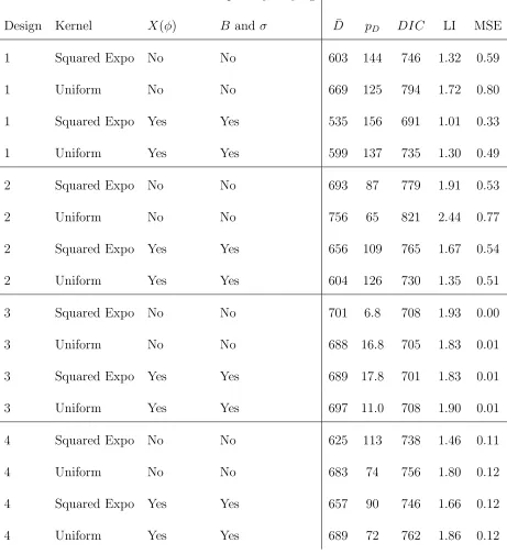
Table 1 gives the results for the four simulated examples. Simulation #3 would
corre-spond to anullmodel, and we would expect, as it is the case, the model comparison statistics
to give a similar answer for the different models. The model comparison statisticsDIC and
LI both select the model with the smallestM SE for simulations #1,#2 and #4, supporting
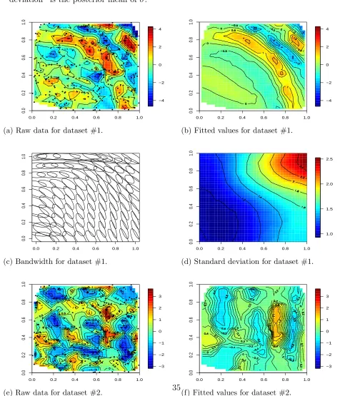
their use for these models. The first simulated data set is clearly anisotropic with stronger
correlation in the northwest/southeast direction and nonstationary with increased variance
in the northeast corner. The nonstationary model with squared-exponential kernel
mini-mizes MSE. The posterior means of the bandwidth and standard deviation for this model in
effects. Both stationary models and the nonstationary model with uniform kernels have
MSE between 0.50 and 0.55 for the second simulated example. The nonstationary model
with uniform kernels gives slightly smaller MSE, possibly due to the elliptical bandwidths
(not shown here) which pool information across nearby undulations with the same heights.
Simulation #4 corresponds to a stationary model, and for both types of kernels, all the
comparison statistics prefer the stationary model.
11
Analysis of speciated PM
2.5In this section we analyze monthly average speciated PM2.5 for January, 2007 at 209
moni-toring stations in the US, plotted in Figure 2. These data were obtained from the US EPA
http://www.epa.gov/airexplorer/index.htm. For our analysis the spatial locations are
transformed to [0,1]2 and the responses are centered and scaled.
We fit several variations of the multivariate spatial stick-breaking model to these data by
varying the kernel (squared-exponential versus uniform), allowing the latentX(s) processes
to have independent or spatial correlation, and allowing the covariance parameters A to be
constant or varying across space with spatial priors. In each of these models we assume the
knots are shared across outcomes and that the kernel bandwidth matrixB is constant across
space and outcome. These nonparametric models are compared to the fully Gaussian model
with stationary, separable covariance
cov(Z(s), Z(s′)) = Σ
e+ exp(ρ|s−s′|)Σ,
where Σe (nugget effect) is the p× p diagonal matrix with diagonal elements σj2 ∼
the p×p cross-covariance matrix.
We compare these models using both the DIC and LI, described in Section 10. In
addition to these model comparisons, we conduct predictive checks of model adequacy using
the Bayesian p-value of Rubin (1984). We compare the replicate data sets with the observed
data Z in terms of a discrepancy measure D(Z). The Bayesian p-value for the discrepancy
measure is
p-value = 1
m
m
X
i=1
I
D(Z)< D(Z(i))
,
where m is the number of MCMC samples. P-values near zero or one indicate that the
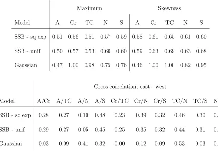
predictive model does not fit the data adequately. We consider several discrepancy measures
including the maximum (over space) D(Z) = max(Z1j, ..., Znj), where Zij denotes Zj(si),
separately for each of the five pollutants, the skewness of each of the five pollutants D(Y) =
skew(Z1j, ..., Znj), and the difference between the cross-correlation of each pair of pollutants
between two locations in the eastern and western halves of the US (see Fig. (12) showing the
location of the pair points), D(Y) = cor(Zij, Zik|i in the east) - cor(Zij, Zik|i in the west).
These measures are chosen to determine, respectively, whether the models adequately capture
tail probabilities, the shape of the response distribution, and the potential non-stationarity
in the cross-covariance between pollutants.
The fully parametric and stationary Gaussian model has the highestDIC andLI of the
models in Table 2. The p-values in Table 3 indicate that the observed data generally have
larger maximums and more skewness than the data sets generated from this model. These
p-values remain unsatisfactory even after a log transformation (not shown), motivating a
east and west are near zero, suggesting non-stationary.
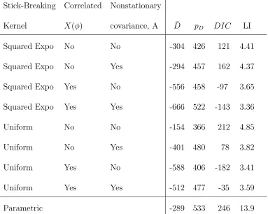
Both DIC and LI are smaller for the nonparametric models in Table 2 than the
para-metric Gaussian model. The most distinguishing factor between the eight nonparapara-metric
models is the correlation of the latent process X(φ); allowing the latent processes to have
spatial correlation improvesDICandLI for all combinations of kernels and cross-covariance
models. The smooth squared-exponential kernels are preferred for the model with
indepen-dentX(φ). In contrast, uniform kernels are preferred whenX(φ) is a spatial process. In this
case, the Gaussian process X(φ) captures large-scale spatial trends and the nonparametric
stick-breaking model with uniform kernels accounts for local spatial effects.
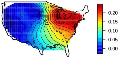
The best-fitting model with squared-exponential kernels allows for nonstationarity in the
cross-covariance. Figure 3 plots the posterior mean and standard deviation of the correlation
between carbon and sulfate and between ammonium and nitrate. Although the standard
deviations of these correlation functions are fairly large, there are clear trends. For example,
the correlation between carbon and sulfate increases from west to east. The Bayesian
p-values for the nonparametric models with spatial correlation in the latent process and
cross-covariance are all between 0.05 and 0.95 (Table 3). This provides evidence that these models
adequately capture the shape of the response distribution and the cross-correlation.
The best-fitting model with uniform kernels has stationary cross-covariance. After
mod-eling the spatial processes adequately with both a Gaussian spatial process X(s) and local
nonparametric model with uniform kernels, the cross-covariance can be taken to be constant
12
Discussion
In this paper we introduce a new modelling nonparametric framework for multivariate
spa-tial processes, that is flexible enough to characterize complex nonstationary dependency and
cross-dependency structures, while avoiding specifying a Gaussian distribution. One of main
advantages of the proposed multivariate spatial stick breaking approach is that is very
com-putationally efficient, and that should be widely useful in situations where several complex
spatial processes need to be modelled simultaneously.
The univariate kernel stick breaking version also provides a useful alternative to recently
developed spatial stick-breaking processes (Griffin and Steel, 2006; Dunson and Park, 2008;
Gelfand et al., 2007; Reich and Fuentes, 2007). One useful feature of this univariate version
is that the limiting process is continuous, rather than discrete as in the other kernel-type
stick breaking approaches.
An advantange of the formulation presented in this paper is that many of the tools
developed for Dirichlet processes can be applied with some modifications, and that has
allowed us to study the statistical properties of the presented methods. The application
presented in this paper is for a multivariate spatial process, but the presented framework
can be applied to multivariate spatial-temporal processes by using space-time kernels. In
our future work, we will implement an extend the presented methods to spatial temporal
References
An, Q., Wang, C., Shterev, I., Wang, E., Carin, L, and Dunson, D. (2008). Hierarchical
kernel stick-breaking process for multi-task image analysis. International Conference
on Machine Learning (ICML), to appear.
Choi J, Reich BJ, Fuentes M, and Davis JM. (2008). Multivariate spatial-temporal modeling
and prediction of speciated fine particles. In press, Journal of Statistical Theory and
Practice.
Dominici, F, Daniels, M, Zeger, S.L, and Samet, J.M., (2002) Air Pollution and
Mortal-ity: Estimating Regional and National Dose-Response Relationships. Journal of the
American Statistical Association,97, 100-111.
Doksum, K. (1974). Tailfree and neutral random probabilities and their posterior d
istri-butions. The Annals of Probability, 2, 183-201
Dunson, D.B. and J. H. Park. (2008). Kernel stick-breaking processes. Biometrika, 95,
307-323.
Gelfand, A.E., A.M. Schmidt, S. Banerjee, and C.F. Sirmans, (2004). Nonstationary
Mul-tivariate Process Modelling through Spatially Varying Coregionalization (with
discus-sion), Test, 13, 2, 1-50.
Gelfand AE, Kottas A, and MacEachern SN (2005). Bayesian nonparametric spatial
mod-eling with Dirichlet process mixing. Journal of the American Statistical Association,
Gelfand, A.E.,Guindani, M., and Petrone, S. (2007). Bayesian nonparametric modeling for
spatial data analysis using Dirichlet processes. Bayesian Statistics, 8. J. Bernardo et
al., eds.
Griffin J.E., and Steel, M.F.J. (2006) Order-based dependent Dirichlet processes. Journal
of the American Statistical Association,101, 179–194.
Laud P., and Ibrahim J. (1995). Predictive model selection. Journal of the Royal Statistical
Society B, 57, 247-262.
Mat´ern, B. (1960). Spatial Variation. Meddelanden fr ˙an Statens Skogsforskningsinstitut,
49, No. 5. Almaenna Foerlaget, Stockholm.
¨
Ozkaynak, H., and Thurston, G. D. (1987), Associations between 1980 U.S. mortality rates
and alternative measures of airborne particle concentration Risk Analysis, 7, 449-461.
Palacios, M.B., and Steel, M.F.J. (2006). Non-Gaussian Bayesian geostatistical modelling.
Journal of the American Statistical Association, Theory and Methods, 101, 604-618.
Papaspiliopoulos O., and Roberts, G. (2008). Retrospective MCMC for Dirichlet process
hierarchical models. Biometrika, 95, 169-186.
Petrone, S., Guindani, M., and Gelfand, A. E. (2008). Hybrid Dirichlet mixture models
for functional data. Tech. report at the Statistics Department at Duke University.
Durham, NC.
Reich B.J., and Fuentes M. (2007). A multivariate semiparametric Bayesian spatial
Sethuraman J. (1994). A constructive definition of Dirichlet priors. Statistica Sinica, 4,
639–650.
Spiegelhalter D.J., Best N.G., Carlin B.P., and van der Linde A. (2002). Bayesian measures
of model complexity and fit (with discussion). Journal of the Royal Statistical Society
B, 64, 583–639.
Song, H.R., Fuentes, M., Ghosh, S. (2008). A comparative study of Gaussian geostatistical
models and Gaussian Markov random field models. Journal of Multivariate analysis,
99, 1681-1697.
Rubin D.B. (1984). Bayesianly justifiable and relevant frequency calculations for the applied
Table 1: Results for the simulated examples.
Correlated Spatially-varying
Design Kernel X(φ) B and σ D¯ pD DIC LI MSE
1 Squared Expo No No 603 144 746 1.32 0.59
1 Uniform No No 669 125 794 1.72 0.80
1 Squared Expo Yes Yes 535 156 691 1.01 0.33
1 Uniform Yes Yes 599 137 735 1.30 0.49
2 Squared Expo No No 693 87 779 1.91 0.53
2 Uniform No No 756 65 821 2.44 0.77
2 Squared Expo Yes Yes 656 109 765 1.67 0.54
2 Uniform Yes Yes 604 126 730 1.35 0.51
3 Squared Expo No No 701 6.8 708 1.93 0.00
3 Uniform No No 688 16.8 705 1.83 0.01
3 Squared Expo Yes Yes 689 17.8 701 1.83 0.01
3 Uniform Yes Yes 697 11.0 708 1.90 0.01
4 Squared Expo No No 625 113 738 1.46 0.11
4 Uniform No No 683 74 756 1.80 0.12
4 Squared Expo Yes Yes 657 90 746 1.66 0.12
Table 2: Model selection results for the speciated PM2.5 data analysis.
Stick-Breaking Correlated Nonstationary
Kernel X(φ) covariance, A D¯ pD DIC LI
Squared Expo No No -304 426 121 4.41
Squared Expo No Yes -294 457 162 4.37
Squared Expo Yes No -556 458 -97 3.65
Squared Expo Yes Yes -666 522 -143 3.36
Uniform No No -154 366 212 4.85
Uniform No Yes -401 480 78 3.82
Uniform Yes No -588 406 -182 3.41
Uniform Yes Yes -512 477 -35 3.59
Table 3: Model adequacy results for the speciated PM2.5 data analysis. The table gives the
Bayesian p-value for three discrepancies: component-wise maximum and skewness, and the
pairwise difference between cross-correlations in the Eastern and Western US. The labels for
the species are “A” for Ammonium, “Cr” crustal materials, “TC” for total carbon, “N” for
nitrate, and “S” for sulfate.
Maximum Skewness
Model A Cr TC N S A Cr TC N S
SSB - sq exp 0.51 0.56 0.51 0.57 0.59 0.58 0.61 0.65 0.61 0.60
SSB - unif 0.50 0.57 0.53 0.60 0.60 0.59 0.63 0.69 0.63 0.68
Gaussian 0.47 1.00 0.98 0.75 0.76 0.46 1.00 1.00 0.82 0.95
Cross-correlation, east - west
Model A/Cr A/TC A/N A/S Cr/TC Cr/N Cr/S TC/N TC/S N/S
SSB - sq exp 0.28 0.27 0.10 0.48 0.23 0.39 0.32 0.46 0.30 0.80
SSB - unif 0.29 0.27 0.05 0.45 0.25 0.35 0.32 0.44 0.31 0.79
Figure 1: Data and results for simulated data set #1 using the nonstationary model with
squared-exponential kernels, and for data set #2 using the nonstationary model with uniform
kernels. The dots are observation locations, “Fitted values” is the posterior mean of the
posterior mean ofPM
i=1pi(sj)X(φi), “bandwidth” is the posterior mean ofBi, and “standard
deviation” is the posterior mean of σ.
0.0 0.2 0.4 0.6 0.8 1.0
0.0 0.2 0.4 0.6 0.8 1.0 −4 −2 0 2 4
0.0 0.2 0.4 0.6 0.8 1.0
0.0 0.2 0.4 0.6 0.8 1.0 −4 −2 0 2 4
(a) Raw data for dataset #1. (b) Fitted values for dataset #1.
0.0 0.2 0.4 0.6 0.8 1.0
0.0 0.2 0.4 0.6 0.8 1.0
0.0 0.2 0.4 0.6 0.8 1.0
0.0 0.2 0.4 0.6 0.8 1.0 1.0 1.5 2.0 2.5
(c) Bandwidth for dataset #1. (d) Standard deviation for dataset #1.
0.0 0.2 0.4 0.6 0.8 1.0
0.0 0.2 0.4 0.6 0.8 1.0 −3 −2 −1 0 1 2 3
0.0 0.2 0.4 0.6 0.8 1.0
Figure 2: Maps of monitoring locations and speciatedP M2.5 data. The two red triangles in
the map with the monitoring locations, show the locations of the pair of points where the
cross-correlation is evaluated.
Monitoring locations Ammonium
1 2 3 4 5 6
Crustal
1 2 3 4
Carbon
5 10 15 20 25
Nitrate
5 10 15
Sulfate
Figure 3: Posterior mean and standard deviation of the spatially-varying cross-correlation
processes.
0.00 0.05 0.10 0.15 0.20
0.15 0.20 0.25 0.30 0.35
(a) Carbon and Sulfate, posterior mean (b) Carbon and Sulfate, posterior sd
0.80 0.85 0.90 0.95
0.10 0.15 0.20 0.25 0.30
1
Appendix
A.1
Properly defined process prior
Kolmogorov existence theorem
We need to prove that the collection of finite-dimensional distributions introduced in
(1) define a stochastic process Y(s). We use the two Kolmogorov consistency conditions
(symmetry under permutation, and dimensional consistency) to show that (1) defines a
proper random process forY.
Proposition 1. The collection of finite-dimensional distributions introduced in (1)
properly define a stochastic process Y(s). We use the two Kolmogorov consistency
con-ditions: symmetry under permutation, and dimensional consistency, to define properly a
random process forY.
Proof of Proposition 1:
Symmetry under permutation.
Let pij = p(Y(sj) = X(φi(sj)), where φi(sj) is the centering knot of the kernel i(sj) in
the representation of Fsj(Y) in (1), and let φij be an abbreviation forφ(i(sj)). Then, pi1,...,in
determine the site-specific joint selection probabilities. If π(1), . . . , π(n) is any permutation
of {1, . . . , n},then we have
piπ(1),...,iπ(n) =p(Y(sπ(1)) =X(φπ(i1)), . . . , Y(sπ(n)) =X(φπ(in)))
since the observations are conditionally independent. Then,
p(Y(s1)∈A1, . . . , Y(sn)∈An)
= X
i1,···,in
p(Y(s1) =X(φi1), . . . , Y(sn) = X(φin))δX(φ(i1))(A1). . . δX(φ(in))(An)
= X
i1,···,in
pi1,...,inδX(φ(i1))(A1). . . δX(φ(in))(An)
= X
i1,···,in
piπ(1),...,iπ(n)δX(φ(iπ(1)))(Aπ(1)). . . δX(φ(iπ(n)))(Aπ(n))
= p(Y(sπ(1))∈Aπ(1), . . . , Y(sπ(n))∈Aπ(n)).
And, the symmetry under permutationcondition holds.
Dimensional consistency.
p(Y(s1)∈(A1), . . . , Y(sk)∈ R, . . . , Y(sn)∈(An))
= X
(i1,...,in)∈{1,2,...}n
pi1,...,inδX(φi1)(A1)· · ·δX(φik)(R)· · ·δX(φin)(An)
= X
(i1,...,ik−1,ik+1,...,in)∈{1,2,...}n−1
δX(φi1)(A1)· · ·δX(φik
−1)(Ak−1)δX(φik+1)(Ak+1)
· · ·δX(φin)(An)
∞ X
j=1
pi1,...,ik−1,j,ik+1,...,in
= p(Y(s1)∈(A1), . . . , Y(sk−1)∈Ak−1, Y(sk+1)∈Ak+1, . . . , Y(sn)∈(An)). (13)
In (13), we need
pi1,...,ik−1,ik+1,...,in =
∞ X
j=1
pi1,...,ik−1,j,ik+1,...,in
which holds by Fubini Theorem and the fact that X is a properly defined Gaussian process.
A.2
The covariance function C of the underlying processX has a first order derivative, C′.
We introduce a Taylor expansion forC with a Lagrange remainder term,
C(|φi1 −φi2|) = C(|s−s
′|) +C′(ψ
i1,i2)εi1,i2, (14)
where εi1,i2 = (|φi1 −φi2| − |s−s
′|) andψ
i1,i2 is in between |s−s
′|and |φ
i1 −φi2|.
Assuming that s and s′ lie on the support of the kernels K
i1 and Ki2, respectively, i.e.
|φi1 −s|< ǫi1 and |φi2 −s ′|< ǫ
i2. We have,
εi1,i2 ≤ ||φi1 −φi2| − |s−s
′|| ≤ |(φ
i1 −φi2)−(s−s ′)| ≤ǫ
i1 +ǫi2 ≤2ǫ,
and,
εi1,i2 ≥ −||φi1 −φi2| − |s−s ′
|| ≥ −|(φi1 −φi2)−(s−s ′
)| ≥ −(ǫi1 +ǫi2)≥ −2ǫ,
Thus, −2ǫ ≤εi1,i2 ≤2ǫ.
Letp(s) be the potentially infinite vector with all the probabilities massespi(s) inFs(Y).
The conditional covariance of the data process Y is written in terms of the covariance C of
X,
cov(Y(s), Y(s′)|p(s), p(s′), C) =X
i1i2
pi1(s)pi2(s ′)C(|φ
i1 −φi2|),
since the kernels all have compact support, the expression above is the same as
X
i1,i2;|φi1−s|<ǫi1,|φi2−s′|<ǫi2
pi1(s)pi2(s ′
)C(|φi1 −φi2|).
Using the Taylor approximation in (14), the cov(Y(s), Y(s′)|p(s), p(s′), C) can be written
C(|s−s′|) "
X
i1
pi1(s) # "
X
i2
pi2(s ′)
#
+ X
i1,i2;|φi1−s|<ǫi1,|φi2−s′|<ǫi2
pi1(s)pi2(s ′)C′(ψ
SinceC′ is nonnegative andε
i1,i2 ∈(−2ǫ,2ǫ),we have that forJi1,i2 ={(i1, i2);|φi1−s|<
ǫi1,|φi2 −s ′|< ǫ
i2},
−2ǫ X
i1,i2∈Ji1,i2
pi1(s)pi2(s ′)C′(ψ
i1,i2) ≤
X
(i1,i2)∈Ji1,i2
pi1(s)pi2(s ′)C′(ψ
i1,i2)εi1,i2
≤ 2ǫ X
(i1,i2)∈Ji1,i2
pi1(s)pi2(s ′)C′(ψ
i1,i2), (15)
where,
2ǫ X
i1,i2∈Ji1,i2
pi1(s)pi2(s ′
)C′(ψi1,i2)−→ǫ→0 0,
because C′ is bounded and the sum of probability masses is always bounded by 1. The sum
of probability masses would be always bounded by 1, because by proposition 1 the prior
process is properly defined.
Thus, we obtain
cov(Y(s), Y(s′)|p(s), p(s′), C)−→ǫ→0 C(|s−s′|)
" X
i1
pi1(s) # "
X
i2
pi2(s ′
)
#
=C(|s−s′|).
Therefore, the conditional covariance of the data process Y approximates the covariance C
of the underlying process X as the bandwiths of the kernel functions go to zero.
A.3
Proof of Theorem 2.
The cross-covariance functionC1,2(s, s′) of the underlying processX = (X1, X2) has first
order partial derivativesδC1,2(s, s′)/δsandδC1,2(s, s′)/δs′. We introduce a Taylor expansion
for C1,2 with a Lagrange remainder term,
C1,2(φi1, φi2) =C1,2(s, s ′
)+(φi1−s) [δC1,2(s, s ′
)/δs](s,s′)=(ψi
1,ψi2)+(φi2−s ′
) [δC1,2(s, s′)/δs′](s,s′)=(ψi
whereψi1 is in between sand φi1, andψi2 is in betweens
′ and φ
i2.We follow the same steps
as in Theorem 1, to bound the first order term of the Taylor expansion, and obtain that
cov(Y1(s), Y2(s′)|p1(s), p2(s′), C1,2)−→ǫ→0 C1,2(s, s′),
wherep1(s),andp2(s′) are the potentially infinite dimensional vectors with the all probability
masses in the spatial stick-breaking prior processes Fs(Y1),and Fs′(Y2) respectively.
A.4
Proof of Theorem 3.
Let ψ(t, s) the characteristic function of Y(s). Then,
ψ(t, s1)−ψ(t, s2) =EY[exp{itY(s1)}]−EY[exp{itY(s2)}]
= EX
( X
j
pj(s1) exp{itX(φj)}
)
−EX
( X
j
pj(s2) exp{itX(φj)}
)
= EX
( X
j
(pj(s1)−pj(s2)) exp{itX(φj)}
)
−→|s1−s2|→0 0. (16)
Then, Fs1(Y) converges to Fs2(Y) for any locations s1, s2, as long as |s1−s2| →0.
A.5
Proof of Theorem 4.
The probability masses pi(s) in (1) are pi(s) = ViKi(s)Qij−=11(1−VjKj(s)). Since the
bandwiths ǫi converge uniformly to zero, then, pi(s) → 1, as |φi −s| → 0, where φi is the
knot of kernel Ki. This holds because Pjpj(s) = 1 a.s. (since the process Y is properly
defined).
Let φ1 and φ2 satisfy,
|φ1−s1| →0, and |φ2−s2| →0. (17)
Thus, we obtain that with probability 1, Y(s1) converges to X(φ1), and Y(s2) to X(φ2).
Since |s1−s2| →0,and |φ1−φ2| ≤ |φ1−s1|+|φ2−s2|+|s1−s2|.Then, by (17)
|φ1−φ2| →0. (18)
We have,
|Y(s1)−Y(s2)| ≤ |Y(s1)−X(φ1)|+|Y(s2)−X(φ2)|+|X(φ1)−X(φ2)|,
where|Y(s1)−X(φ1)| →0 a.s., as|s1−φ1| →0;|Y(s2)−X(φ2)| →0 a.s., as|s2−φ2| →0;
and since X is a.s. continuous, |X(φ1)−X(φ2)| →0 a.s., as|φ1−φ2| → 0 (which holds by
18).