Locally Adaptive Factor Processes for Multivariate Time Series

Locally Adaptive Factor Processes

for Multivariate Time Series

Daniele Durante [email protected]

Bruno Scarpa [email protected]

Department of Statistical Sciences University of Padua

Padua 35121, Italy

David B. Dunson [email protected]

Department of Statistical Science Duke University

Durham, NC 27708-0251, USA

Editor:Robert E. McCulloch

Abstract

In modeling multivariate time series, it is important to allow time-varying smoothness in the mean and covariance process. In particular, there may be certain time intervals exhibiting rapid changes and others in which changes are slow. If such time-varying smoothness is not accounted for, one can obtain misleading inferences and predictions, with over-smoothing across erratic time intervals and under-smoothing across times exhibiting slow variation. This can lead to mis-calibration of predictive intervals, which can be substantially too narrow or wide depending on the time. We propose a locally adaptive factor process for characterizing multivariate mean-covariance changes in continuous time, allowing locally varying smoothness in both the mean and covariance matrix. This process is constructed utilizing latent dictionary functions evolving in time through nested Gaussian processes and linearly related to the observed data with a sparse mapping. Using a di↵erential equation representation, we bypass usual computational bottlenecks in obtaining MCMC and online algorithms for approximate Bayesian inference. The performance is assessed in simulations and illustrated in a financial application.

Keywords: Bayesian nonparametrics, locally varying smoothness, multivariate time se-ries, nested Gaussian process, stochastic volatility

1. Introduction

over-2004-07-19 2006-02-18 2007-09-21 2009-04-22 2010-11-23 2012-06-25

0.00

0.01

0.02

0.03

0.04

0.05

0.06

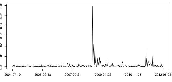
DAX30: Squared log returns

Figure 1: Squared log returns of DAX30. Weekly data from 19/07/2004 to 25/06/2012.

smoothing during times of rapid change. This leads to an under-estimation of uncertainty during such volatile times and an inability to accurately predict risk of extremal events.

Let yt = (y1t, . . . , ypt)T denote a random vector at time t, with µ(t) = E(yt) and

⌃(t) = cov(yt). Our focus is on Bayesian modeling and inference for the multivariate

mean-covariance stochastic process, ={µ(t),⌃(t), t2T } with T ⇢ <+_{. Of particular interest} is allowing locally varying smoothness, meaning that the rate of change in the_{µ(t),⌃(t)_} process is varying over time. To our knowledge, there is no previous proposed stochastic process for a coupled mean-covariance process, which allows locally varying smoothness. A key to our construction is the use of latent processes, which have time-varying smoothness. This results in a locally adaptive factor (LAF) process. We review the relevant literature below and then describe our LAF formulation.

1.1 Relevant Literature

Johnstone, 1995), local polynomial fitting via variable bandwidth (Fan and Gijbels, 1995) and linear combination of kernels with variable bandwidths (Wolpert et al., 2011).

There is a separate literature on estimating a time-varying covariance matrix ⌃(t). This is particularly of interest in applications where volatilities and co-volatilities evolve through non constant paths. One popular approach estimates ⌃(t) via an exponentially weighted moving average (EWMA); see, e.g., Tsay (2005). This approach uses a single time-constant smoothing parameter 0 < < 1, with extensions to accommodate locally varying smoothness not straightforward due to the need to maintain positive semidefinite ⌃(t) at every time. To allow for higher flexibility in the dynamics of the covariances, generalizations of EWMA have been proposed including the diagonal vector ARCH model (DVEC), (Bollerslev et al., 1988) and its variant, the BEKK model (Engle and Kroner, 1995). These models are computationally demanding and are not designed for moderate to largep. DCC-GARCH (Engle, 2002) improves the computational tractability of the previous approaches through a two-step formulation. However, the univariate GARCH assumed for the conditional variances of each time series and the higher level GARCH models with the same parameters regulating the evolution of the time-varying conditional correlations, restrict the evolution of the variance and covariance matrices. PC-GARCH (Ding, 1994; Burns, 2005) and O-GARCH (Alexander, 2001) perform dimensionality reduction through a latent factor formulation; see also van der Weide (2002). However, time-constant factor loadings and uncorrelated latent factors constrain the evolution of⌃(t).

Such models fall far short of our goal of allowing ⌃(t) to be fully flexible with the dependence between ⌃(t) and⌃(t+ ) varying with not just the time-lag but also with time. In addition, these models do not handle missing data easily and tend to require long series for accurate estimation (Burns, 2005). Accommodating changes in continuous time is important in many applications, and avoids having the model be critically dependent on the time scale, with inconsistent models obtained as time units are varied.

Wilson and Ghahramani (2010) join machine learning and econometrics e↵orts by propos-ing a model for both mean and covariance regression in multivariate time series, improvpropos-ing previous work of Bru (1991) on Wishart processes in terms of computational tractability and scalability, allowing a more complex structure of dependence between ⌃(t) and ⌃(t+ ). Specifically, they propose a continuous time generalised Wishart process (GWP), which defines a collection of positive semi-definite random matrices⌃(t) with Wishart marginals. Nonparametric mean regression forµ(t) is also considered via GP priors; however, the tra-jectories of means and covariances inherit the smooth behavior of the underlying Gaussian processes, limiting the flexibility of the approach across times exhibiting sharp changes.

a latent thresholding approach, leading to apparently improved performance in portfolio al-location. They assume a time-varying discrete-time autoregressive model, which allows the dependence in the covariance matrices⌃(t) and⌃(t+ ) to vary as a function of bothtand . However, the result is a richly parameterized and computationally challenging model, with selection of the number of factors proceeding by cross validation. Our emphasis is instead on developing continuous time stochastic processes for⌃(t) andµ(t), which accom-modate locally varying smoothness and provide relatively efficient MCMC computations based on a Gibbs sampler.

Fox and Dunson (2011) propose an alternative Bayesian covariance regression (BCR) model, which defines the covariance matrix as a regularized quadratic function of time-varying loadings in a latent factor model, characterizing the latter as a sparse combination of a collection of unknown Gaussian process dictionary functions. Although their approach provides a continuous time and highly flexible model that accommodates missing data and scales to moderately largep, there are two limitations motivating this article. Firstly, their proposed covariance stochastic process assumes a stationary dependence structure, and hence tends to under-smooth during periods of stability and over-smooth during periods of sharp changes. Secondly, the well known computational problems with usual GP regression are inherited, leading to difficulties in scaling to long series and issues in mixing of MCMC algorithms for posterior computation.

1.2 Contribution and Outline

Our proposed LAF process instead includes dictionary functions that are generated from nested Gaussian processes (nGP) (Zhu and Dunson, 2013), representing recently proposed priors which exploit stochastic di↵erential equations (SDEs) to enforce GP priors for the function’s mth order derivatives and favor local adaptivity by centering the latter on an higher level GP instantaneous mean. Such nGP reduces the GP computational burden involving matrix inversions from O(T3_{) to O(T), with T denoting the length of the time} series, while also allowing flexible locally varying smoothness. Marginalizing out the latent factors, we obtain a stochastic process that inherits these advantages. We also develop a di↵erent and more computationally efficient approach under this new model and propose an online implementation, which can accommodate streaming data. In Section 2, we describe the LAF structure with particular attention to prior specification. Section 3 explores the main features of the Gibbs sampler for posterior computation and outlines the steps for a fast online updating approach. In Section 4 we compare our model to BCR and to some of the most widely used models for multivariate stochastic volatility, through simulation studies. Finally in Section 5 an application to National Stock Market Indices across countries is examined.

2. Locally Adaptive Factor Processes

Our focus is on defining a novel locally adaptive factor process for ={µ(t),⌃(t), t2T }. In particular, taking a Bayesian approach, we define a prior _⇠P, whereP is a probability measure over the space _P ofp-variate mean-covariance processes on_T. In particular, each element of P corresponds to a realization of the stochastic process , and the measure P

Although the proposed class of LAF processes can be used much more broadly, in conducting inferences in this article, we focus on the simple case in which data consist of vectors yi = (y1i, . . . , ypi)T collected at times ti, for i = 1, . . . , T. These times can be

unequally-spaced, or collected under an equally-spaced design with missing observations. An advantage of using a continuous-time process is that it is trivial to allow unequal spacing, missing data, and even observation times across which only a subset of the elements of yi

are observed. We additionally make the simplifying assumption that

yi ⇠Np(µ(ti),⌃(ti)).

It is straightforward to modify the methodology to accommodate substantially di↵erent observation models.

2.1 LAF Specification

A common strategy in modeling of large p matrices is to rely on a lower-dimensional fac-torization, with factor analysis providing one possible direction. Sparse Bayesian factor models have been particularly successful in challenging cases, while having advantages over frequentist competitors in incorporating a probabilistic characterization of uncertainty in the number of factors as well as the parameters in the loadings and residual covariance. For recent articles on Bayesian sparse factor analysis for a single large covariance matrix, refer to Bhattacharya and Dunson (2011), Pati et al. (2012) and the references cited therein.

In our setting, we are instead interested in letting the mean vector and the covariance matrix vary flexibly over time. Extending the usual factor analysis framework to this setting, we say that =_{µ(t),⌃(t), t_{2T }⇠}LAFL,K(⇥,⌃0,⌃⇠,⌃A,⌃ ,⌃B) if

µ(t) =⇥⇠(t) (t), (1a)

⌃(t) =⇥⇠(t)⇠(t)T⇥T +⌃0, (1b) where⇥is ap_⇥Lmatrix of constant coefficients,⌃0 = diag( 12, . . . , p2), while⇠(t)L⇥K and

(t)K⇥1 are matrices comprising continuous dictionary functions evolving in time via nGP,

⇠lk(t)⇠nGP([⌃⇠]lk = ⇠2lk,[⌃A]lk =

2

Alk) and k(t)⇠nGP([⌃ ]k= 2_k,[⌃B]k= 2Bk).

Restricting our attention on the generic element ⇠lk(t) : T ! < of the matrix ⇠(t)L⇥K

(the same holds for k(t) :T ! <), the nGP provides a highly flexible stochastic process on

the dictionary functions whose smoothness, explicitly modeled by their mth order deriva-tives Dm⇠lk(t) via stochastic di↵erential equations, is expected to be centered on a local

instantaneous mean functionAlk(t), which represents a higher-level Gaussian process, that

induces adaptivity to locally varying smoothing. Specifically, we let

Dm⇠lk(t) =Alk(t) + ⇠lkW⇠lk(t), m2N, m 2, (2a)

DnAlk(t) = AlkWAlk(t), n2N, n 1, (2b)

where ⇠lk 2 <

+_,

Alk 2 <+, W⇠lk(t) : T ! < and WAlk(t) : T ! < are independent

Gaussian white noise processes with mean E[W⇠lk(t)] = E[WAlk(t)] = 0, for all t2T, and

covariance function E[W⇠lk(t)W⇠lk(t⇤)] = E[WAlk(t)WAlk(t⇤)] = 1 if t = t⇤, 0 otherwise.

where E[Dm_⇠

lk(t)|Alk(t)] =Alk(t), and initialization at t1 based on the assumption [⇠lk(t1), D1⇠lk(t1), . . . , Dm 1⇠lk(t1)]T ⇠ Nm(0, 2µlkIm),

[Alk(t1), D1Alk(t1), . . . , Dn 1Alk(t1)]T ⇠ Nn(0, ↵2lkIn).

The Markovian property implied by SDEs in (2a) and (2b) represents a key advantage in terms of computational tractability as it allows a simple state space formulation. In particular, referring to Zhu and Dunson (2013) for m = 2 and n = 1 (this can be easily extended for higher mand n), and for i =ti+1 ti sufficiently small, the process for⇠lk(t)

along with its first order derivative ⇠_lk0 (t) and the local instantaneous mean Alk(t) follow

the approximated state equation

" _⇠

lk(ti+1)

⇠_lk0 (ti+1)

Alk(ti+1) #

=

"

1 i 0

0 1 i

0 0 1

# " _⇠ lk(ti) ⇠_lk0 (ti) Alk(ti)

# + " 0 0 1 0 0 1 #_h !i,⇠lk !i,Alk

i

, (3)

where [!i,⇠lk,!i,Alk]

T _{⇠N2(0, V}

i,lk), withVi,lk = diag( 2⇠lk i,

2

Alk i).

Similarly to the nGP specification for the elements in⇠(t), we can represent the nested Gaussian process for k(t) with the following state equation:

"

k(ti+1) 0

k(ti+1)

Bk(ti+1)

#

=

" ₁

i 0

0 1 i

0 0 1

# " k(ti)

0

k(ti) Bk(ti)

#

+

" _{0 0}

1 0 0 1

#_h !i, k !i,Bk

i

, (4)

fork = 1, . . . , K, where [!i, k,!i,Bk]

T _⇠N

2(0, Si,k), with Si,k = diag( 2_k i, 2Bk i).

Simi-larly to ⇠lk(t), we let

[ k(t1), D1 k(t1), . . . , Dm 1 k(t1)]T ⇠ Nm(0, 2µkIm),

[Bk(t1), D1Bk(t1), . . . , Dn 1Bk(t1)]T ⇠ Nn(0, ↵2kIn).

There are two crucial aspects to highlight. Firstly, this formulation is defined at every point over a subset of the real line and allows an irregular grid of observations over t by relating the latent states at i+ 1 to those at i through the distance between ti+1 and ti where i represents a discrete order index and ti 2 T the time value related to the ith

observation. Secondly, compared to Zhu and Dunson (2013) our approach represents an important generalization in: (i) extending the analysis to the multivariate case (i.e. yi is a p-dimensional vector instead of a scalar) and (ii) accommodating locally adaptive smoothing not only on the mean but also on the time-varying covariance functions.

2.2 LAF Interpretation

Model (1a)–(1b) can be induced by marginalizing out the K-dimensional latent factors vector⌘i, in the model

yi=⇤(ti)⌘i+✏i, ✏i⇠Np(0,⌃0), (5)

where ⌘i = (ti) +⌫i with ⌫i ⇠ NK(0, IK) and elements k(t) ⇠ nGP( 2_k, 2Bk) for k =

matrix⇤(t) is a sparse linear combination, with respect to the weights of thep_⇥Lmatrix ⇥, of a much smaller set of continuous nested Gaussian processes ⇠lk(t) ⇠nGP( ⇠2lk,

2

Alk)

comprising theL_⇥K, with L << p, matrix ⇠(t). As a result

⇤(ti) =⇥⇠(ti). (6)

Such a decomposition plays a crucial role in further reducing the number of nested Gaussian processes to be modeled fromp_⇥K toL_⇥K leading to a more computationally tractable formulation in which the induced =_{µ(t),⌃(t), t_{2T }}follows a locally adaptive factor LAFL,K(⇥,⌃0,⌃⇠,⌃A,⌃ ,⌃B) process where

µ(ti) = E(yi |t=ti) =⇥⇠(ti) (ti), (7a)

⌃(ti) = cov(yi |t=ti) =⇥⇠(ti)⇠(ti)T⇥T +⌃0. (7b) There is a literature on using Bayesian factor analysis with time-varying loadings, but essentially all the literature assumes discrete-time dynamics on the loadings while our focus is instead on allowing the loadings, and hence the induced =_{µ(t),⌃(t), t_{2T }}processes, to evolve flexibly in continuous time. Hence, we are most closely related to the literature on Gaussian process latent factor models for spatial and temporal data; refer, for example, to Lopes et al. (2008) and Lopes et al. (2011). In these models, the factor loadings matrix characterizes spatial dependence, with time-varying factors accounting for dynamic changes. Fox and Dunson (2011) instead allow the loadings matrix to vary through a continuous time stochastic process built from latent GP(0, c) dictionary functions independently for all

l = 1, . . . , L and k = 1, . . . , K, with c the squared exponential correlation function having

c(t, t⇤) = exp( _||t t⇤_||2

2). In our work we follow the lead of Fox and Dunson (2011) in using a nonparametric latent factor model as in (5)–(6), but induce fundamentally di↵erent behavior on =_{µ(t),⌃(t), t_{2T }} by carefully modifying the stochastic processes for the dictionary functions.

Note that the above decomposition of =_{µ(t),⌃(t), t_{2T }} is not unique. Potentially we could constrain the loadings matrix to enforce identifiability (Geweke and Zhou, 1996), but this approach induces an undesirable order dependence among the responses (Aguilar and West, 2000; West, 2003; Lopes and West, 2004; Carvalho et al., 2008). Given our focus on estimation of we follow Ghosh and Dunson (2009) in avoiding identifiability constraints, as such constraints are not necessary to ensure identifiability of the induced meanµ(t) and covariance⌃(t). The characterization of the class of time-varying covariance matrices ⌃(t) is proved by Lemma 2.1 of Fox and Dunson (2011) which states that for K

and L sufficiently large, any covariance regression can be decomposed as in (1b). Similar results are obtained for the mean process.

2.3 Prior Specification

We adopt a hierarchical prior specification approach to induce a priorP on =_{µ(t),⌃(t), t₂ T } with the goal of maintaining simple computation and allowing both covariances and means to evolve flexibly over continuous time. Specifically

• Recalling the assumption ⇠lk(t) ⇠ nGP( _⇠2_lk, 2_Alk) within LAF representation, we

assume for each each element [⌃⇠]lk and [⌃A]lk of the L⇥K matrices ⌃⇠ and ⌃A

respectively, the following priors 2

⇠lk ⇠ InvGa(a⇠, b⇠),

2

Alk ⇠ InvGa(aA, bA),

independently for each (l, k); where InvGa(a, b) denotes the Inverse Gamma distribu-tion with shape aand scaleb.

• Similarly, the variances [⌃ ]k= 2_k and [⌃B]k= Bk2 in the state equation

represen-tation of the nGP for each k(t)⇠nGP( 2_k, B2k) are assumed

2

k ⇠ InvGa(a , b ),

2

Bk ⇠ InvGa(aB, bB),

independently for each k.

• To address the issue related to the selection of the number of dictionary elements a shrinkage prior is proposed for ⇥. In particular, following Bhattacharya and Dunson (2011) we assume

✓_jl| jl,⌧l ⇠N(0, _jl1⌧_l 1), jl⇠Ga(3/2,3/2),

#1⇠Ga(a1,1), #h⇠ Ga(a2,1), h 2, ⌧l=

l Y

h=1

#h. (8)

Note that if a2 > 1 the expected value for #h is greater than 1. As a result, as l

goes to infinity,⌧ltends to infinity, shrinking✓jl towards zero. This leads to a flexible

prior for✓jlwith a local shrinkage parameter jl and a global column-wise shrinkage

factor ⌧l which allows many elements of ⇥ being close to zero as L increases. Our

formulation can be easily generalized to allow shrinkage over K; see Fox and Dunson (2011). However we found reasonable to fixK to relatively small values and learn L

with the shrinkage approach, to avoid higher computational complexity in sampling theK-variate vector (ti), i= 1, . . . , T.

• Finally for the variances of the error terms in vector✏i, we assume the usual inverse

gamma prior distribution. Specifically 2

j ⇠Ga(a , b )

independently for each j= 1, . . . , p.

3. Posterior Computation

3.1 Gibbs Sampling

We outline here the main features of the algorithm for posterior computation based on observations (yi, ti) for i= 1, . . . , T, while the complete algorithm is provided in Appendix

A. Note that, since data are in practice observed at a finite number of times, the continuous time model is approximated in conducting inferences. This issue arises in analyzing data with any continuous time model.

A. Given⇥and {⌘i}Ti=1, a multivariate version of the MCMC algorithm proposed by Zhu and Dunson (2013) draws posterior samples from each dictionary element’s function

{⇠lk(ti)}Ti=1, its first order derivative {⇠lk0 (ti)}Ti=1, the corresponding instantaneous mean{Alk(ti)}Ti=1, the variances in the state equations ⇠2lk,

2

Alk and the variances of

the error terms in the observation equation 2

j with j= 1, . . . , p.

B. Given⇥,{ j 2} p

j=1,{yi}Ti=1and{⇠(ti)}Ti=1we implement a block sampling of{ k(ti)}Ti=1,

{ 0

k(ti)}Ti=1,{Bk(ti)}Ti=1, 2k,

2

Bk and ⌫i following a similar approach as in step A.

C. Conditioned on _{y_i}T

i=1,{⌘i}Ti=1, { j 2} p

j=1 and {⇠(ti)}Ti=1, and recalling the shrinkage prior for the elements of⇥in (8), we update⇥, each local shrinkage hyperparameter

jl and the global shrinkage hyperparameters ⌧l following the standard conjugate

analysis.

D. Given the posterior samples from ⇥, ⌃0, {⇠(ti)}iT=1 and { (ti)}Ti=1 the realization of LAF process for _{µ(ti),⌃(ti), ti 2T } conditioned on the data {yi}Ti=1 is

µ(ti) = ⇥⇠(ti) (ti),

⌃(ti) = ⇥⇠(ti)⇠(ti)T⇥T +⌃0. 3.2 Hyperparameters Interpretation

We now focus our attention on the priors hyperparameters for 2_⇠lk, 2_Alk, 2_kand 2_Bk. These quantities play an important role in facilitating local adaptivity and carefully tuning such values may improve mixing and convergence speed of our MCMC algorithm. Simulation studies have shown that the higher the variances in the latent state equations, the better our formulation accommodates locally adaptivity for sudden changes in . A theoretical support for this data-driven consideration can be identified in the connection between the nGP and the nested smoothing splines. It has been shown by Zhu and Dunson (2013) that the posterior mean of the trajectoryU with reference to the problem of nonparametric mean regression under the nGP prior can be related to the minimizer of the equation

1

T T X

i=1

(yi U(ti))2+ U Z

T

(DmU(t) C(t))2dt+ C Z

T

(DnC(t))2dt,

where C is the locally instantaneous function and U 2 <+ and C 2 <+ regulate the

smoothness of the unknown functionsU and C respectively, leading to less smoothed pat-terns when fixed at low values. The resulting inverse relationship between these smoothing parameters and the variances in the state equation, together with the results in the simula-tion studies, suggest to fix the hyperparameters in the Inverse Gamma prior for 2_⇠

lk,

2

2

k and

2

Bk so as to allow high variances in the case in which the time series analyzed are

expected to have strong changes in their covariance (or mean) dynamic. A further confir-mation of the previous discussion is provided by the structure of the simulation smoother required to update the dictionary functions in our Gibbs sampling for posterior computa-tion. More specifically, the larger the variances of {!i,⇠lk}Ti=1, {!i,Alk}Ti=1 and {!i, k}

T i=1,

{!_i,Bk}T_i=1in the state equations, with respect to those of the vector of observations_{y_i}T_i=1,

the higher is the weight associated to innovations in the filtering and smoothing techniques, allowing for less smoothed patterns both in the covariance and mean structures (see Durbin and Koopman, 2002).

In practical applications, it may be useful to obtain a first estimate of ˜ ={µ˜(t),⌃(˜ t)}

to set the hyperparameters. More specifically, ˜µj(ti) can be the output of a standard moving

average on each time series yj = (yj1, . . . , yjT)T, while ˜⌃(ti) can be obtained by a simple

estimator, such as the EWMA procedure. With these choices, the recursive equation

˜

⌃(ti) = (1 ){[yi 1 µ˜(ti 1)][yi 1 µ˜(ti 1)]T}+ ˜⌃(ti 1), become easy to implement.

3.3 Online Updating

The problem of online updating represents a key point in multivariate time series with high frequency data. Referring to our formulation, we are interested in updating an approximated posterior for T+H = {µ(tT+h),⌃(tT+h), h = 1, . . . , H} once a new vector of observations {y_i}T_i=+_TH₊₁is available, instead of rerunning posterior computation for the whole time series. Using the posterior estimates of the Gibbs sampler based on observations available up to time T, it is easy to implement (see Appendix B) a highly computationally tractable online updating algorithm which alternates between steps A, B and D outlined in the previous section for the new set of observations, and that can be initialized at T+ 1 using the one step ahead predictive distribution for the latent state vectors in the state space formulation. Such initialization procedure for latent state vectors in the algorithm depends on the sample moments of the posterior distribution for the latent states at T. As is known for Kalman smoothers (see, e.g., Durbin and Koopman, 2001), this could lead to computational problems in the online updating due to the larger conditional variances of the latent states at the end of the sample (i.e., atT). To overcome this problem, we replace the previous assumptions for the initial values with a data-driven initialization scheme. In particular, instead of using only the new observations for the online updating, we run the algorithm for {yi}Ti=+T kH , withk small. As a result the distribution of the smoothed states

atT is not anymore a↵ected by the problem of large conditional variances leading to better online updating performance.

of the time-constant parameters and if the number of time series analyzed p is tractable. Since we search for a relatively fast procedure, and provided that for moderately largeT the posterior for the time-stationary parameters rapidly becomes concentrated, we preferred our initially proposed algorithm in order to avoid thepdraws from anL⇤ dimensional Gaussian in the sampling of⇥, which may slow down the online updating procedure for largep.

4. Simulation Studies

The aim of the following simulation studies is to compare the performance of our pro-posed LAF with respect to BCR, and to the models for multivariate stochastic volatility most widely used in practice, specifically: EWMA, PC-GARCH, GO-GARCH and DCC-GARCH. In order to assess whether and to what extent LAF can accommodate, in practice, even sharp changes in the time-varying means and covariances and to evaluate the costs of our flexible approach in settings where the mean and covariance functions do not require locally adaptive estimation techniques, we focus on two di↵erent sets of simulated data. The first is based on an underlying structure characterized by locally varying smoothness processes, while the second has means and covariances evolving in time through smooth processes. In the last subsection we also analyze the performance of the proposed online updating algorithm.

4.1 Simulated Data

A. Locally varying smoothness processes: We generate a set of 5-dimensional observations

yi for each ti in the discrete set To = {1,2, . . . ,100}, from the latent factor model

in (5) with ⇤(ti) = ⇥⇠(ti). To allow sharp changes of means and covariances in

the generating mechanism, we consider a 2⇥2 (i.e. L = K = 2) matrix {⇠(ti)}100i=1 of time-varying functions adapted from Donoho and Johnstone (1994) with locally varying smoothness (more specifically we choose ‘bumps’ functions). The latent mean dictionary elements in{ (ti)}100i=1are simulated from a Gaussian process GP(0, c) with length scale= 10, while the elements in matrix⇥can be obtained from the shrinkage prior in (8) witha1 =a2 = 10. Finally the elements of the diagonal matrix ⌃01 are sampled independently from Ga(1,0.1).

B. Smooth processes: We consider the same data set of 10-dimensional observations yi

with ti 2 To = {1,2, . . . ,100} investigated in Fox and Dunson (2011, Section 4.1).

The settings are similar to the previous with exception of{⇠(ti)}100i=1 which are 5⇥4 matrices of smooth GP dictionary functions with length scale= 10.

4.2 Estimation Performance

A. Locally varying smoothness processes:

Posterior computation for LAF is performed by using truncation levelsL⇤ =K⇤= 2 (at higher level settings we found that the shrinkage prior on ⇥ results in posterior samples of the elements in the additional columns concentrated around 0). We place a Ga(1,0.1) prior on the precision parameters _j2 and choose a1 =a2 = 2. As regards the nGP prior for each dictionary element⇠lk(t) withl= 1, . . . , L⇤ andk= 1, . . . , K⇤,

and place an InvGa(2,108_{) prior on each} 2

⇠lk and

2

Alk in order to allow less smooth

behavior according to a previous graphical analysis of ˜⌃(ti) estimated via EWMA.

Similarly we set _µk2 = 2_↵k = 100 in the prior for the initial values of the latent state equations resulting from the nGP prior for k(t), and considera =aB=b =bB=

0.005 to balance the rough behavior induced on the nonparametric mean functions by the settings of the nGP prior on⇠lk(t), as suggested from previous graphical analysis.

Note also that for posterior computation, we first scale the predictor space to (0,1], leading to i= 1/100,fori= 1, . . . ,100.

For inference in BCR we consider the same previous hyperparameters setting for ⇥ and⌃0 priors as well as the same truncation levelsK⇤ andL⇤, while the length scale

 in GP prior for ⇠lk(t) and k(t) has been set to 10 using the data-driven heuristic

outlined in Fox and Dunson (2011). In both cases we run 50,000 Gibbs iterations discarding the first 20,000 as burn-in and thinning the chain every 5 samples.

As regards the other approaches, EWMA has been implemented by choosing the smoothing parameter that minimizes the mean squared error (MSE) between the estimated covariances and the true values. PC-GARCH algorithm follows the steps provided by Burns (2005) with GARCH(1,1) assumed for the conditional volatilities of each single time series and the principal components. GO-GARCH and DCC-GARCH recall the formulations provided by van der Weide (2002) and Engle (2002) respectively, assuming a GARCH(1,1) for the conditional variances of the processes analyzed, which proves to be a correct choice in many financial applications and also in our setting. Note that, di↵erently from LAF and BCR, the previous approaches do not model explicitly the mean process_{µ(ti)}100i=1but work directly on the innovations{yi µ(ti)}100i=1. Therefore in these cases we first model the conditional mean via smoothing spline and in a second step we estimate the models working on the innovations. The smoothing parameter for spline estimation has been set to 0.7, which was found to be appropriate to best reproduce the true dynamic of {µ(ti)}100

i=1. B. Smooth processes:

We mainly keep the same setting of the previous simulation study with few di↵erences. Specifically, L⇤ and K⇤ has been fixed to 5 and 4 respectively (also in this case the choice of the truncation levels proves to be appropriate, reproducing the same results provided in the simulation study of Fox and Dunson (2011) where L⇤ = 10 and

K⇤ = 10). Moreover the scale parameters in the Inverse Gamma prior on each _⇠2

lk

and 2

Alk has been set to 104 in order to allow a smoother behavior according to a

previous graphical analysis of ˜⌃(ti) estimated via EWMA, but without forcing the

nGP prior to be the same as a GP prior. Following Fox and Dunson (2011) we run 10,000 Gibbs iterations which proved to be enough to reach convergence, and discarded the first 5,000 as burn-in.

Time

0 20 40 60 80 100

0

50

100

150

Time

0 20 40 60 80 100

-3 00 -2 50 -2 00 -1 50 -1 00 -5 0 0 Time

0 20 40 60 80 100

-6 -4 -2 0 2 4

0 20 40 60 80 100

1

2

3

4

5

0 20 40 60 80 100

-0 .5 0.0 0.5 1.0 1.5

0 20 40 60 80 100

-0 .4 -0 .2 0.0 0.2 0.4 0.6 0.8 1.0

⌃2,2(ti)

⌃1,3(ti) µ5(ti)

⌃9,9(ti) ⌃10,3(ti) µ5(ti)

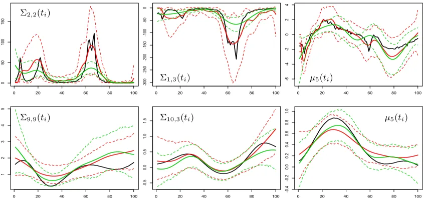
Figure 2: For locally varying smoothness simulation (top) and smooth simulation (bottom), plots of truth (black) and posterior mean respectively of LAF (solid red line) and BCR (solid green line) for selected components of the variance (left), covariance (middle), mean (right). For both approaches the dotted lines represent the 95% highest posterior density intervals.

BCR the 95% quantile is 1.44 and the median equals 1.18. Less problematic is the mixing for the second set of simulated data, with potential scale reduction factors having median equal to 1.05 for both approaches and 95% quantiles equal to 1.15 and 1.31 for LAF and BCR, respectively.

Figure 2 compares, in both simulated samples, true and posterior mean of the process

= _{µ(ti),⌃(ti), i = 1, . . . ,100} over the predictor space To together with the point-wise

Mean 90% Quantile 95% Quantile Max Covariance _{⌃(ti)}

EWMA 1.37 2.28 5.49 85.86 PC-GARCH 1.75 2.49 6.48 229.50 GO-GARCH 2.40 3.66 10.32 173.41 DCC-GARCH 1.75 2.21 6.95 226.47 BCR 1.80 2.25 7.32 142.26 LAF 0.90 1.99 4.52 36.95

Mean_{µ(ti)}

SPLINE 0.064 0.128 0.186 2.595 BCR 0.087 0.185 0.379 2.845 LAF 0.062 0.123 0.224 2.529

Table 1: LOCALLY VARYING SMOOTHNESS PROCESSES: Summaries of the standard-ized squared errors between true values _{µ(ti)}100i=1 and {⌃(ti)}100i=1 and estimated quantities{⌃(ˆ ti)}100

i=1 and {µˆ(ti)}100i=1 computed with di↵erent approaches. Mean 90% Quantile 95% Quantile Max

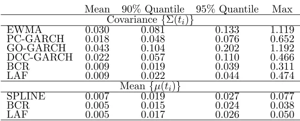
Covariance _{⌃(ti)}

EWMA 0.030 0.081 0.133 1.119 PC-GARCH 0.018 0.048 0.076 0.652 GO-GARCH 0.043 0.104 0.202 1.192 DCC-GARCH 0.022 0.057 0.110 0.466 BCR 0.009 0.019 0.039 0.311 LAF 0.009 0.022 0.044 0.474

Mean_{µ(ti)}

SPLINE 0.007 0.019 0.027 0.077 BCR 0.005 0.015 0.024 0.038 LAF 0.005 0.017 0.026 0.050

Table 2: SMOOTH PROCESSES: Summaries of the standardized squared errors between true values {µ(ti)}100

i=1 and {⌃(ti)}100i=1 and estimated quantities {⌃(ˆ ti)}100i=1 and

{µˆ(ti)}100i=1 computed with di↵erent approaches.

The comparison of the summaries of the squared errors between true process =

{µ(ti),⌃(ti), i= 1, . . . ,100} and the estimated quantities ˆ = {µˆ(ti),⌃(ˆ ti), i = 1, . . . ,100}

standardized with the range of the true processes rµ= maxi,j{µj(ti)} mini,j{µj(ti)} and r⌃ = maxi,j,k{⌃j,k(ti)} mini,j,k{⌃j,k(ti)}respectively, once again confirms the overall

bet-ter performance of our approach relative to all the considered competitors. Table 1 shows that, when local adaptivity is required, LAF provides a superior performance having stan-dardized residuals lower than those of the other approaches. EWMA seems to provide quite accurate estimates, but it is important to underline that we choose the optimal smoothing parameter in order to minimize the MSE between estimated and true parameters, which are clearly not known in practical applications. Di↵erent values of reduces significantly the performance of EWMA, which shows also lack of robustness. The closeness of the sum-maries of LAF and BCR in Table 2 confirms the flexibility of LAF even in settings where local adaptivity is not required and highlights the better performance of the two approaches with respect to the other competitors also when smooth processes are investigated.

0 20 40 60 80 100

-1

5

-5

0

5

10

15

20

Series 1

time

0 20 40 60 80 100

-1

0

0

10

20

Series 2

time

0 20 40 60 80 100

-4

0

-2

0

0

10

20

30

Series 3

0 20 40 60 80 100

-4

0

-2

0

0

10

20

30

Series 4

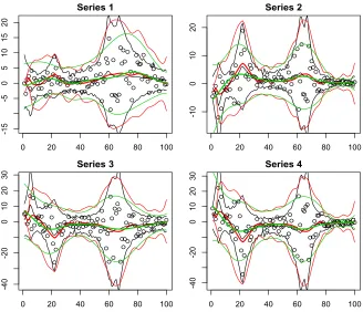
Figure 3: For 4 selected simulated series: time-varying mean µj(ti) and 2.5% and 97.5%

quantiles of the marginal distribution ofyji with true mean and variance (black),

mean and variance from posterior mean of LAF (red), mean and variance from posterior mean of BCR (green). Black points represent the simulated data.

distribution ofyi withi= 1, . . . ,100 consider Figure 3 which shows, for some selected series {y_ji}100

i=1 in the first simulated data set, the time-varying mean together with the point-wise 2.5% and 97.5% quantiles of the marginal distribution of yji induced respectively by the true mean and true variance, the posterior mean of µj(ti) and ⌃jj(ti) from our proposed

approach and the posterior mean of the same quantities from BCR. We can clearly see that the marginal distribution of yji induced by BCR is over-concentrated near the mean, leading to incorrect inferences. Note that our proposal is also able to accommodate heavy tails, a typical characteristic in financial series.

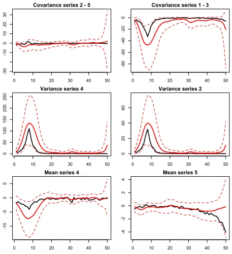
4.3 Online Updating Performance

To analyze the performance of the online updating algorithm in LAF model, we simulate 50 new observations {yi}150

i=101 with ti 2To⇤ ={101, . . . ,150}, considering the same ⇥ and

⌃0 used in the generating mechanism for the first simulated data set and taking the 50 subsequent observations of the bumps functions for the dictionary elements _{⇠(ti)}150i=101; finally the additional latent mean dictionary elements{ (ti)}150

Covariance series 2 - 5

Time

0 10 20 30 40 50

-3

0

-1

0

0

10

20

30

Covariance series 1 - 3

Time

0 10 20 30 40 50

-8

0

-6

0

-4

0

-2

0

0

Variance series 4

Time

0 10 20 30 40 50

0

50

100

150

200

250

Variance series 2

Time

0 10 20 30 40 50

0

20

40

60

Mean series 4

0 10 20 30 40 50

-1

0

-5

0

5

Mean series 5

0 10 20 30 40 50

-4

-2

0

2

4

Figure 4: Plots of truth (black) and posterior mean of the online updating procedure (solid red line) for selected components of the covariance (top), variance (middle), mean (bottom). The dotted lines represent the 95% highest posterior density intervals.

the algorithm described in Subsection 3.3, we fix⇥,⌃0,⌃⇠,⌃A,⌃ and⌃Bat their posterior

mean from the previous Gibbs sampler and consider the last three observationsy98,y99and

y100(i.e. k= 3) to initialize the simulation smoother ini= 101 through the proposed data-driven initialization approach. Posterior computation shows good performance in terms of mixing, and convergence is assessed after 5,000 Gibbs iterations with a small burn-in of 500. Figure 4 compares true mean and covariance to posterior mean of a selected set of components of _⇤ = _{µ(ti),⌃(ti), i = 101, . . . ,150} including also the 95% hpd intervals.

The results clearly show that the online updating is characterized by a good performance which allows to capture the behavior of new observations conditioning on the previous estimates. Note that the posterior distribution of the approximated mean and covariance functions tends to slightly over-estimate the patterns of the functions at sharp changes, however also in these cases the true values are within the bands of the credibility intervals. Finally note that the data-driven initialization ensures a good behavior at the beginning of the series, while the results at the end have wider uncertainty bands as expected.

5. Application Study

followed in recent years, we applied our LAF to the multivariate time series of the main National Stock Market Indices.

5.1 National Stock Market Indices, Introduction and Motivation

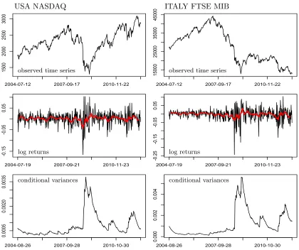
National Stock Market Indices represent technical tools that allow, through the synthesis of numerous data on the evolution of the various stocks, to detect underlying trends in the financial market, with reference to a specific basis of currency and time. More specifically, each Market Index can be defined as a weighted sum of the values of a set of national stocks, whose weighting factors is equal to the ratio of its market capitalization in a specific date and overall of the whole set on the same date.

In this application we focus our attention on the multivariate weekly time series of the main 33 (i.e. p = 33) National Stock Market Indices from 12/07/2004 to 25/06/2012. Figure 5 shows the main features in terms of stationarity, mean patterns and volatility of two selected National Stock Market Indices downloaded from http://finance.yahoo. com/. The non-stationary behavior, together with the di↵erent bases of currency and time, motivate the use of logarithmic returns yji = log(Iji/Iji 1), where Iji is the value of the Stock Market Index j at time ti. Beside this, the marginal distribution of log returns

shows heavy tails and irregular cyclical trends in the nonparametric estimation of the mean, while EWMA estimates highlight rapid changes of volatility during the financial crises observed in the recent years. All these results, together with large p settings and high frequency data typical in financial fields, motivate the use of our approach to obtain a better characterization of the time-varying dependence structure among financial markets.

5.2 LAF for National Stock Market Indices

We consider the heteroscedastic modelyi ⇠N33(µ(ti),⌃(ti)) fori= 1, . . . ,415 andti in the

discrete set _To = _{1,2, . . . ,415_}, where the elements of = _{µ(ti),⌃(ti), i = 1, . . . ,415},

defined by (7a)-(7b), are induced by the dynamic latent factor model outlined in (5)-(6). Posterior computation is performed by first rescaling the predictor space_Toto (0,1] and using the same setting of the first simulation study, with the exception of the truncation levels fixed at K⇤ = 4 and L⇤ = 5 (which we found to be sufficiently large from the fact that the last few columns of the posterior samples for ⇥ assumed values close to 0) and the hyperparameters of the nGP prior for each⇠lk(t) and k(t) withl= 1, . . . , L⇤ and k=

1, . . . , K⇤, set to a⇠ =aA=a =aB= 2 andb⇠ =bA=b =bB= 5⇥107 to capture also

rapid changes in the mean functions according to Figure 5. Missing values in our data set do not represent a limitation since the Bayesian approach allows us to update our posterior considering solely the observed data. We run 10,000 Gibbs iterations with a burn-in of 2,500. Examination of trace plots of the posterior samples for = _{µ(ti),⌃(ti), i = 1, . . . ,415}

showed no evidence against convergence.

Time

2004-07-12 2007-09-17 2010-11-22

1500

2000

2500

3000

Time

2004-07-12 2007-09-17 2010-11-22

15000

25000

35000

45000

Time

2004-07-19 2007-09-21 2010-11-23

-0

.1

5

-0

.0

5

0.05

Time

2004-07-19 2007-09-21 2010-11-23

-0

.2

5

-0

.1

5

-0

.0

5

0.05

2004-08-26 2007-09-28 2010-10-30

0.0005

0.0020

0.0035

TS.

1

2004-08-260.000 2007-09-28 2010-10-30

0.002

0.004

USA NASDAQ ITALY FTSE MIB

observed time series observed time series

log returns log returns

conditional variances conditional variances

Figure 5: Plots of the main features of USA NASDAQ (left) and ITALY FTSE MIB (right). Specifically: observed time series (top), log returns series with nonparametric mean estimation via 12 week Equally Weighted Moving Average (red) in the middle, EWMA volatility estimates (bottom).

the resulting marginal distribution of the log returns induced by the posterior mean ofµj(t)

and⌃jj(t), shows that we are also able to accommodate heavy tails as well as mean patterns

cycling irregularly between slow and more rapid changes.

Time

2004-07-19 2007-09-21 2010-11-23

-0

.1

5

-0

.0

5

0.05

0.10

Time

2004-07-19 2007-09-21 2010-11-23

-0

.2

-0

.1

0.0

0.1

2004-07-190.000 2007-09-21 2010-11-23

0.002

0.004

0.006

2004-07-190.000 2007-09-21 2010-11-23

0.002

0.004

0.006

USA NASDAQ ITALY FTSE MIB

log returns log returns

conditional variances conditional variances

Figure 6: Top: Plot for 2 National Stock Market Indices, respectively USA NASDAQ (left) and ITALY FTSE MIB (right), of the log returns (black) and the time-varying estimated mean{µjˆ (ti)}415

i=1together with the time-varying 2.5% and 97.5% quan-tiles (red) of the marginal distribution ofyji from LAF. Bottom: posterior mean

(black) and 95% hpd (dotted red) for the variances_{⌃jj(ti)}415i=1.

in terms of geographical, political and economic structure; the same holds for Eastern countries where we observe a reversal of the colored curves. As expected, Russia is placed in a middle path between the two blocks. A further element that our model captures about the structure of the markets is shown in the plots at the bottom of Figure 8. The time-varying regression coefficients obtained from the standard formulas of the conditional normal distribution based on the posterior mean of = _{µ(ti),⌃(ti), i = 1, . . . ,415} highlight

clearly the increasing dependence of European countries with higher crisis in sovereign debt and Germany, which plays a central role in Eurozone as expected.

0.0

0.2

0.4

0.6

0.8

A B C D E F G

2004-07-19 2005-12-05 2007-04-23 2008-09-08 2010-01-25 2011-06-13

2004-07-19 2005-12-05 2007-04-23 2008-09-08 2010-01-25 2011-06-13

0.2

0.4

0.6

0.8

A B C D E F G

2004-07-19 2005-12-05 2007-04-23 2008-09-08 2010-01-25 2011-06-13

2004-07-19 2005-12-05 2007-04-23 2008-09-08 2010-01-25 2011-06-13

LAF

BCR

Figure 7: Black line: For USA NASDAQ median of correlations with the other 32 National Stock Market Indices based on posterior mean of {⌃(ti)}415i=1. Red lines: 25%, 75% (dotted lines) and 50% (solid line) quantiles of correlations between USA NASDAQ and European countries (without considering Greece and Russia which present a specific pattern). Green lines: 25%, 75% (dotted lines) and 50% (solid line) quantiles of correlations between USA NASDAQ and the countries of South-east Asia (Asian Tigers and India). Timeline: (A) burst of U.S. housing bubble; (B) risk of failure of the first U.S. credit agencies (Bear Stearns, Fannie Mae and Freddie Mac); (C) world financial crisis after the Lehman Brothers’ bankruptcy; (D) Greek debt crisis; (E) financial reform launched by Barack Obama and E.U. e↵orts to save Greece (the two peaks represent respectively Irish debt crisis and Portugal debt crisis); (F) worsening of European sovereign-debt crisis and the rejection of the U.S. budget; (G) crisis of credit institutions in Spain and the growing financial instability of the Eurozone.

Time

0.2

0.4

0.6

0.8

2004-07-19 2006-05-152008-03-10 2010-01-04 2011-10-31

Time

-0

.1

0.0

0.1

0.2

0.3

0.4

0.5

2004-07-192006-05-15 2008-03-10 2010-01-042011-10-31

Time

0.0

0.2

0.4

0.6

0.8

2004-07-192006-05-15 2008-03-102010-01-04 2011-10-31

2004-07-19 2007-09-21 2010-11-23

0.00

0.05

0.10

0.15

2004-07-19 2007-09-21 2010-11-23

0.00

0.05

0.10

0.15

2004-07-19 2007-09-21 2010-11-23

-0

.0

5

0.00

0.05

0.10

GERMANY DAX30 CHINA SSE Composite RUSSIA RTSI Index

ITALY SPAIN GREECE

Figure 8: Top: For 3 selected National Stock Market Indices, plot of the median of the correlation based on posterior mean of _{⌃(ti)}415i=1 with the other 32 world stock indices (black), the European countries without considering Greece and Russia (red) and the Asian Tigers including India (green). Bottom: For 3 of the Eu-ropean countries more subject to sovereign debt crisis, plot of 25%, 50% and 75% quantiles of the time-varying regression parameters based on posterior mean

{⌃(ˆ ti)}415i=1 with the other countries (black) and Germany (red).

can notice two peaks representing respectively Irish debt crisis and Portugal debt crisis. Note also that BCR, as expected, tends to over-smooth the dynamic dependence structure during the financial crisis, proving to be not able to model the sharp change in the corre-lations between USA NASDAQ and Economic Tigers during late-2008, and the two peaks representing respectively Irish and Portugal debt crisis at the beginning of 2011.

5.3 National Stock Market Indices, Updating and Predicting

The possibility to quickly update the estimates and the predictions as soon as new data arrive, represents a crucial aspect to obtain quantitative informations about the future scenarios of the crisis in financial markets. To answer this goal, we apply the online updating algorithm presented in Subsection 3.3, to the new set of weekly observations_{y_i}422_i=416 from 02/07/2012 to 13/08/2012 conditioning on posterior estimates of the Gibbs sampler based on observations{yi}415

Time -0 .0 5 0.00 0.05

2012-07-02 2012-07-16 2012-07-30 2012-08-13

Time -0 .0 5 0.00 0.05 0.10

2012-07-02 2012-07-16 2012-07-30 2012-08-13

Time -0 .0 5 0.00 0.05 0.10

2012-07-02 2012-07-16 2012-07-30 2012-08-13

(a)

2012-07-02 2012-07-16 2012-07-30 2012-08-13

(b)

2012-07-02 2012-07-16 2012-07-30 2012-08-13

(c)

2012-07-02 2012-07-16 2012-07-30 2012-08-13

USA NASDAQ INDIA BSE30 FRANCE CAC40

Figure 9: Top: For 3 selected National Stock Market Indices, respectively USA NASDAQ (left), INDIA BSE30 (middle) and FRANCE CAC40 (right), plot of the ob-served log returns (black) together with the mean and the 2.5% and 97.5% quan-tiles of the marginal distribution (red) and conditional distribution given the other 32 National Stock Market Indices (green) based on the posterior mean of ⇤ ={µ(ti),⌃(ti), i= 416, . . . ,422} from the online updating procedure for the

new observations from 02/07/2012 to 13/08/2012. Bottom: boxplots of the one step ahead prediction errors for the 33 National Stock Market Indices, where the predicted values are respectively: (a) unconditional mean _{y˜i+1}421i=415 = 0, (b) marginal mean of the one step ahead predictive distribution, (c) conditional mean given the log returns of the other 32 NSI at i+ 1 of the one step ahead predictive distribution. Predictions for (b) and (c) are induced by the posterior mean of{µ(ti+1|i),⌃(ti+1|i), i= 415, . . . ,421}of LAF.

Plots at the top of Figure 9 show, for 3 selected National Stock Market Indices, the new observed log returns _{y_ji}422

i=416 (black) together with the mean and the 2.5% and 97.5% quantiles of the marginal distribution (red) and conditional distribution (green) ofyji|y_i j

withy_i j ={yqi, q6=j}. We use standard formulas of the multivariate normal distribution

based on the posterior mean of the updated _⇤=_{µ(ti),⌃(ti), i= 416, . . . ,422} after 5,000

To obtain further informations about the predictive performance of our LAF, we can easily use our online updating algorithm to obtain h step-ahead predictions for T+H|T =

{µ(t_T+h|T),⌃(t_T+h|T), h = 1, . . . , H_}. In particular, referring to Durbin and Koopman

(2001), we can generate posterior samples of _T+H|T merely by treating_{y_i}T_i=+_TH₊₁as missing values in the proposed online updating algorithm. Here, we consider the one step ahead prediction (i.e. H = 1) problem for the new observations. More specifically, for eachifrom 415 to 421, we update the mean and covariance functions conditioning on informations up toti through the online algorithm and then obtain the predicted posterior distribution for

⌃(ti+1|i) and µ(ti+1|i) by adding to the sample considered for the online updating a last

columnyi+1 of missing values.

Plots at the bottom of Figure 9, show the boxplots of the one step ahead prediction errors for the 33 National Stock Market Indices obtained as the di↵erence between the predicted value ˜yj,i+1 and, once available, the observed log return yj,i+1 with i+ 1 = 416, . . . ,422 corresponding to weeks from 02/07/2012 to 13/08/2012. In (a) we forecast the future log returns with the unconditional mean _{y˜i+1}421i=415 = 0, which is what is often done in practice under the general assumption of zero mean, stationary log returns. In (b) we consider ˜yi+1 = ˆµ(ti+1|i), the posterior mean of the one step ahead predictive distribution of µ(t_i+1|i), obtained from the previous proposed approach after 5,000 Gibbs iteration with a burn in of 500. Finally in (c) we suppose that the log returns of all National Stock Market Indices except that of country j (i.e., yj,i+1) become available at ti+1 and, considering

y_{i+1|i ⇠} Np(ˆµ(ti+1|i),⌃(ˆ ti+1|i)) with ˆµ(ti+1|i) and ˆ⌃(ti+1|i) posterior mean of the one step

ahead predictive distribution respectively forµ(t_i+1|i) and⌃(t_i+1|i), we forecastyj,i+1 with the conditional mean ofyj,i+1|igiven the other log returns at timeti+1. Comparing boxplots in (a) with those in (b) we can see that our model allows to obtain improvements also in terms of prediction. Furthermore, by analyzing the boxplots in (c) we can notice how our ability to obtain a good characterization of the time-varying covariance structure can play a crucial role also in improving forecasting, since it enters into the standard formula for calculating the conditional mean in the normal distribution.

6. Discussion

In this paper, we have presented a continuous time multivariate stochastic process for time series to obtain a better characterization for mean and covariance temporal dynamics. Maintaining simple conjugate posterior updates and tractable computations in moderately largep settings, our model increases significantly the flexibility of previous approaches as it captures sharp changes both in mean and covariance dynamics while accommodating heavy tails. Beside these key advantages, the state space formulation enables development of a fast online updating algorithm particularly useful for high frequency data.

The simulation studies highlight the flexibility and the overall better performance of LAF with respect to the models for multivariate stochastic volatility most widely used in practice, both when adaptive estimation techniques are required, and also when the underlying mean and covariance structures do not show sharp changes in their dynamic.

reference to (i) heavy tails, (ii) locally adaptive mean regression, (iii) sharp changes in co-variance functions, (iii) high dimensional data set, (iv) online updating with high frequency data (v) missing values and (vi) predictions. Potentially further improvements are possible using a stochastic di↵erential equation model that explicitly incorporates prior information on dynamics.

Acknowledgments

This research was partially supported by grant R01ES17240 from the National Institute of Environmental Health Sciences (NIEHS) of the National Institutes of Health (NIH) and by grant CPDA121180/12 from the University of Padua, Italy.

Appendix A. Posterior Computation

For a fixed truncation level L⇤ and a latent factor dimensionK⇤ the detailed steps of the Gibbs sampler for posterior computations are:

1. Define the vector of the latent states and the error terms in the state space equation resulting from nGP prior for dictionary elements as

⌅i = [⇠11(ti),⇠21(ti), . . . ,⇠L⇤_K⇤(t_i),⇠₁₁0 (t_i), . . . ,⇠0_L⇤K⇤(ti), A11(ti), . . . , AL⇤_K⇤(t_i)]T,

⌦i,⇠ = [!i,⇠11,!i,⇠21, . . . ,!i,⇠L⇤K⇤,!i,A11,!i,A21, . . . ,!i,AL⇤K⇤] T_.

Given ⇥, {⌘i}T

i=1, {yi}Ti=1, ⌃0 and the variances in latent state equations { ⇠2lk},

{ 2

Alk}, withl= 1, . . . , L⇤ andk= 1, . . . , K⇤; update{⌅i}Ti=1 by using the simulation smoother in the following state space model

yi = [⌘iT ⌦⇥,0p⇥(2⇥K⇤_⇥L⇤₎]⌅i+✏i, (9)

⌅i+1 = Ti⌅i+Ri⌦i,⇠, (10)

where the observation equation in (9) results by applying thevecoperator in the latent factor modelyi =⇥⇠(ti)⌘i+✏i. More specifically recalling the propertyvec(ABC) =

(CT _{⌦A)vec(B) we obtain}

yi = vec(yi) = vec{⇥⇠(ti)⌘i+✏i}

= vec{⇥⇠(ti)⌘i}+vec(✏i) = (⌘_iT ⌦⇥)vec{⇠(ti)}+✏i.

The state equation in (10) is a joint representation of the equations resulting from the nGP prior on each⇠lk(t) defined in (3). As a result, the (3⇥L⇤⇥K⇤)⇥(3⇥L⇤⇥K⇤)

ma-trixTitogether with the (3⇥L⇤⇥K⇤)⇥(2⇥L⇤⇥K⇤) matrixRireproduce, for each dic-tionary element the state equation in (3) by fixing to 0 the coefficients relating latent states with di↵erent (l, k) (from the independence between the dictionary elements). Finally, recalling the assumptions on!i,⇠lkand!i,Alk,⌦i,⇠is normally distributed with

E[⌦i,⇠] = 0 and E[⌦i,⇠⌦Ti,⇠] = diag( 2⇠11 i, . . . , 2⇠L⇤K⇤ i,

2

A11 i, . . . ,

2

2. Given_{⌅_i}T

i=1 sample each ⇠2lk and

2

Alk respectively from

2

⇠lk|{⌅i} ⇠ InvGa a⇠+ T

2, b⇠+ 1 2

T 1

X

i=1

(⇠_lk0 (ti+1) ⇠lk0 (ti) Alk(ti) i)2 i

! ,

2

Alk|{⌅i} ⇠ InvGa aA+ T

2, bA+ 1 2

T 1

X

i=1

(Alk(ti+1) Alk(ti))2 i

! .

3. Similarly to ⌅i and ⌦i,⇠ let

i = [ 1(ti), 2(ti), . . . , K⇤(ti), 01(ti), . . . , K0 ⇤(ti), B1(ti), . . . , BK⇤(ti)]T,

⌦i, = [!i, 1,!i, 2, . . . ,!i, K⇤,!i,B1,!i,B2, . . . ,!i,BK⇤] T_,

be the vectors of the latent states and error terms in the state space equation resulting from nGP prior for (t). Conditional on⇥,{⇠(ti)}T

i=1,{yi}Ti=1,⌃0, and the variances in latent state equations { 2

k},{

2

Bk}, with k= 1, . . . , K⇤; sample{ i}Ti=1 from the simulation smoother in the following state space model

yi = [⇥⇠(ti),0p⇥(2⇥K⇤₎] i+$i, (11)

i+1 = Gi i+Fi⌦i, , (12)

$i ⇠N(0,⇥⇠(ti)⇠(ti)T⇥T+⌃0). The observation equation in (11) results by marginal-izing out ⌫i in the latent factor model with nonparametric mean regression yi = ⇥⇠(ti) (ti) +⇥⇠(ti)⌫i+✏i. Analogously to ⌅i, the state equation in (12) is a joint

representation of the state equation induced by the nGP prior on each k(t) defined in

(4); where the (3⇥K⇤)⇥(3⇥K⇤) matrixGi and the (3⇥K⇤)⇥(2⇥K⇤) matrixFiare constructed with the same goal of the matricesTi andRi in the state space model for

⌅i. Finally, ⌦i, ⇠N2⇥K⇤(0,diag( ₁2 i, ₂2 i, . . . , 2_K⇤ i, 2B1 i,

2

B2 i, . . . ,

2

BK⇤ i)).

4. Given{ i}T

i=1 update each 2k and

2

Bk respectively from

2

k|{ i} ⇠ InvGa a + T

2, b + 1 2

T_X1

i=1

( 0_k(ti+1) _k0(ti) Bk(ti) i)2 i

! ,

2

Bk|{ i} ⇠ InvGa aB+ T

2, bB+ 1 2

T_X1

i=1

(Bk(ti+1) Bk(ti))2 i

! .

5. Conditioned on⇥,⌃0,yi,⇠(ti) and (ti), and recalling⌫i ⇠NK⇤(0, IK⇤); the standard

conjugate posterior distribution⌫i|⇥,⌃0,yi,˜ ⇠(ti), (ti) is

NK⇤ (I+⇠(t_i)T⇥T⌃₀1⇥⇠(t_i)) 1⇠(t_i)T⇥T⌃₀1y˜_i,(I+⇠(t_i)T⇥T⌃₀1⇥⇠(t_i)) 1 ,

6. Conditioned on ⇥,_{⌘_i}T

i=1, {yi}Ti=1, and{⇠(ti)}Ti=1 (obtained from ⌅i), the standard

conjugate posterior from which to update _j2 is

2

j |⇥,{⌘i},{yi},{⇠(ti)}⇠Ga a + T

2, b + 1 2

T X

i=1

(yji ✓j_·⇠(ti)⌘i)2

! .

Where✓j·= [✓j1, . . . ,✓jL⇤]

7. Given_{⌘_i}T

i=1,{yi}Ti=1,{⇠(ti)}Ti=1and the hyperparameters and⌧ the shrinkage prior on ⇥ combined with the likelihood for the latent factor model lead to the Gaussian posterior

✓j·|{⌘i},{yi},{⇠(ti)}, ,⌧ ⇠NL⇤ ⌃˜_✓⌘˜T _j2

" yj1

. . . yjT # ,⌃˜✓ ! ,

where ˜⌘T _{= [⇠(t}

1)⌘1,⇠(t2)⌘2, . . . ,⇠(tT)⌘T] and

˜

⌃_✓1 = _j 2⌘˜T⌘˜+ diag( j1⌧1, . . . , jL⇤⌧L⇤).

8. The Gamma prior on the local shrinkage hyperparameter jl implies the standard

conjugate posterior given ✓jl and ⌧l

jl|✓jl,⌧l⇠Ga 2,

3 +⌧l✓jl2

2 .

!

9. Conditioned on⇥ and⌧, sample the global shrinkage hyperparameters from

#1|⇥,⌧( 1) ⇠Ga

0 @a1+

pL⇤

2 ,1 + 1 2

L⇤

X

l=1

⌧_l( 1) p X

j=1

jl✓2jl 1 A,

#h|⇥,⌧( h)⇠Ga 0 @a2+

p(L⇤ h+ 1)

2 ,1 + 1 2

L⇤ X

l=h ⌧_l( h)

p X

j=1

jl✓jl2 1 A,

where⌧_l( h) =Ql_t=1,t6=h#tforh= 1, . . . , L⇤.

10. Given the posterior samples from ⇥,⌃0, {⇠(ti)}T

i=1 and { (ti)}Ti=1 the realization of the LAF process for _{µ(ti),⌃(ti), ti2T }conditioned on the data {yi}Ti=1 is

µ(ti) = ⇥⇠(ti) (ti),

Appendix B. Online Updating Algorithm

Consider⇥,⌃0,{ 2

⇠lk},{

2

Alk},{ 2k}and{

2

Bk}fixed at their posterior mean ˆ⇥, ˆ⌃0,{ˆ⇠2lk}, {ˆ2_Alk}, {ˆ2

k},{ˆ

2

Bk} respectively, and let ˆ⌅T, ˆ⌃⌅T and ˆT, ˆ⌃ T be the sample mean and

covariance matrix of the posterior distribution respectively for ⌅T and T obtained from

the posterior estimates of the Gibbs sampler conditioned on{yi}T i=1.

1. Given ˆ⇥, ˆ⌃0,{ˆ_⇠2_lk},{ˆ2_Alk},{⌘i}Ti=+TH+1 and{yi}Ti=+TH+1 update{⌅i}Ti=+TH+1 by using the simulation smoother in the following state space model

yi = [⌘_iT ⌦⇥ˆ,0p⇥(2⇥K⇤_⇥L⇤)]⌅i+✏i,

⌅i+1 = Ti⌅i+Ri⌦i,⇠,

where⌅T+1can be initialized from the standard one step ahead predictive distribution for the state space model ⌅T+1⇠N(TT⌅ˆT, TT⌃ˆ⌅TTTT +RTE[⌦T,⇠⌦T_T,⇠]RTT).

2. Conditioned on ˆ⇥, ˆ⌃0,{ˆ2_k},{ˆ_Bk2 }, {⇠(ti)}iT=+TH+1 and {yi}iT=+TH+1 sample { i}Ti=+TH+1 through the simulation smoother in the state space model

yi = [ ˆ⇥⇠(ti),0p⇥(2⇥K⇤)] i+$i,

i+1 = Gi i+Fi⌦i, .

Similarly to⌅T+1, T+1 ⇠N(GTˆT, GT⌃ˆ TG T

T +FTE[⌦T, ⌦TT, ]FTT).

3. Given ˆ⇥, ˆ⌃0, {yi}, ⇠(ti) and (ti), for i = T + 1, . . . , T +H, sample ⌫i from the

standard conjugate posterior distribution for⌫i|⇥ˆ,⌃0ˆ ,yi,˜ ⇠(ti), (ti):

NK⇤

⇣

(I+⇠(ti)T⇥ˆT⌃ˆ01⇥ˆ⇠(ti)) 1⇠(ti)T⇥ˆT⌃ˆ01y˜i,(I+⇠(ti)T⇥ˆT⌃ˆ01⇥ˆ⇠(ti)) 1 ⌘

,

with ˜yi =yi ⇥ˆ⇠(ti) (ti).

4. Compute the updated covariance_{⌃(ti)}Ti=+TH+1 and mean{µ(ti)}Ti=+TH+1from the usual equations

⌃(ti) = ⇥ˆ⇠(ti)⇠(ti)T⇥ˆT + ˆ⌃0,

µ(ti) = ⇥ˆ⇠(ti) (ti).

References

O. Aguilar and M. West. Bayesian dynamic factor models and portfolio allocation. Journal

of Business & Economic Statistics, 18(3):338–357, 2000.

C.O. Alexander. Orthogonal GARCH. Mastering Risk, 2:21–38, 2001.

A. Bhattacharya and D.B. Dunson. Sparse Bayesian infinite factor models. Biometrika, 98(2):291–306, 2011.

T. Bollerslev, R.F. Engle and J.M. Wooldridge. A capital-asset pricing model with time-varying covariances. Journal of Political Economy, 96(1):116–131, 1988.

M. Bru. Wishart Processes. Journal of Theoretical Probability, 4(4):725–751, 1991.

P. Burns. Multivariate GARCH with Only Univariate Estimation. Available electronically

athttp://www.burns-stat.com/pages/Working/multgarchuni.pdf, 2005.

C.M. Carvalho, J.E. Lucas, Q. Wang, J. Chang, J.R. Nevins and M. West. High-dimensional sparse factor modeling - Applications in gene expression genomics. Journal of the

Amer-ican Statistical Association, 103(484):1438–1456, 2008.

S. Claessens and K. Forbes. International Financial Contagion. Springer, New York, 2001.

Z. Ding. Time series analysis of speculative returns. PhD thesis, University of California, San Diego, 1994.

D.L. Donoho and J.M. Johnstone. Ideal spatial adaptation by wavelet shrinkage.

Biometrika, 81(3):425–455, 1994.

D.L. Donoho and J.M. Johnstone. Adapting to unknown smoothness via wavelet shrinkage.

Journal of the American Statistical Association, 90(432):1200–1224, 1995.

J. Durbin and S. Koopman.Time Series Analysis by State Space Methods. Oxford University Press Inc., New York, 2001.

J. Durbin and S. Koopman. A simple and efficient simulation smoother for state space time series analysis. Biometrika, 89(3):603–615, 2002.

R.F. Engle and K.F. Kroner. Multivariate simultaneous generalized ARCH. Econometric

Theory, 11(1):122–150, 1995.

R.F. Engle. Dynamic conditional correlation: a simple class of multivariate generalized autoregressive conditional heteroskedasticity models. Journal of Business & Economic

Statistics, 20(3):339–350, 2002.

J. Fan and I. Gijbels. Data-driven bandwidth selection in local polynomial fitting: variable bandwidth and spatial adaptation. Journal of the Royal Statistical Society. Series B, 57(2):371–394, 1995.

E. Fox and D.B. Dunson. Bayesian Nonparametric Covariance Regression. Available elec-tronically at http://arxiv.org/pdf/1101.2017.pdf, 2011.

J.H. Friedman. Multivariate Adaptive Regression Splines. Annals of Statistics, 19(1):1–67, 1991.

A. Gelman and D.B. Rubin. Inference from iterative simulation using multiple sequences.

E.I. George and R.E. McCulloch. Variable selection via Gibbs sampling. Journal of the

American Statistical Association, 88(423):881–889, 1993.

J. Geweke and G. Zhou. Measuring the pricing error of the arbitrage pricing theory.Review

of Financial Studies, 9(2):557–587, 1996.

J. Ghosh and D.B. Dunson. Default Prior Distributions and Efficient Posterior Compu-tation in Bayesian Factor Analysis. Journal of Computational and Graphical Statistics, 18(2):306–320, 2009.

T.J. Hastie and R.J. Tibshirani. Generalized Additive Models. Chapman & Hall, London, 1990.

J.Z. Huang, C.O. Wu and L. Zhou. Varying-coefficient models and basis function approxi-mations for the analysis of repeated measurements. Biometrika, 89(1):111–128, 2002.

R.E. Kalman. A new approach to linear filtering and prediction problems. Journal of Basic

Engineering , 82(1):35–45, 1960.

H.F. Lopes and C.M. Carvalho. Factor stochastic volatility with time-varying loadings and Markov switching regimes. Journal of Statistical Planning and Inference, 137(10):3082– 3091, 2007.

H.F. Lopes, D. Gamerman and E. Salazar. Generalized spatial dynamic factor models.

Computational Statistics & Data Analysis, 55(3):1319–1330, 2011.

H.F. Lopes, E. Salazar and D. Gamerman. Spatial Dynamic Factor Analysis. Bayesian

Analysis, 3(4):759–792, 2008.

H.F. Lopes and M. West. Bayesian model assessment in factor analysis. Statistica Sinica, 14(1):41–67, 2004.

J. Nakajima and M. West. Bayesian analysis of latent threshold dynamic models. Journal

of Business and Economic Statistics, 31(2):151–164, 2013.

D. Pati, A. Bhattacharya, N.S. Pillai and D.B. Dunson. Bayesian high-dimensional co-variance matrix estimation. Available electronically at http://ftp.stat.duke.edu/

WorkingPapers/12-05.html, 2012.

C.E. Rasmussen and C.K.I Williams. Gaussian processes for machine learning. MIT Press, Boston, 2006.

B.W. Silverman. Spline Smoothing: The Equivalent Variable Kernel Method. Annals of

Statistics, 12(3):898-916, 1984.

M. Smith and R. Kohn. Nonparametric regression using Bayesian variable selection.Journal

of Econometrics, 75(2):317-343, 1996.

R. van der Weide. GO-GARCH: a multivariate generalized orthogonal GARCH model.

Journal of Applied Econometrics, 17(5):549–564, 2002.

M. West. Bayesian factor regression models in the largep, smallnparadigm. InProceedings

of the Seventh Valencia International Meeting, pages 723–732, Tenerife, Spain, 2003.

A.G. Wilson and Z. Ghahramani. Generalised Wishart Processes. Available electronically

athttp://arxiv.org/pdf/1101.0240.pdf, 2010.

R.L. Wolpert, M.A. Clyde and C. Tu. Stochastic expansions using continuous dictionaries: Levy adaptive regression kernels. Annals of Statistics, 39(4):1916–1962, 2011.

C.O. Wu, C.T. Chiang and D.R. Hoover. Asymptotic confidence regions for kernel smooth-ing of a varysmooth-ing-coefficient model with longitudinal data. Journal of the American

Sta-tistical Association, 93(444):1388-1402, 1998.