ABSTRACT
YARMAND, HAMED. Optimizing Intervention Strategies and Resource Allocation for Infectious Diseases. (Under the direction of Dr. Julie S. Ivy and Dr. Alun L. Lloyd.)
The focus of this research is the identification of optimal intervention strategies in case of an epidemic caused by an infectious disease. In the first step, we consider the susceptible-infective (SI) epidemiological model, a variant of the Kermack-McKendrick models, and let the contact rate be a function of the number of infectives, an indicator of disease spread during the course of the epidemic. We represent the resultant model as a continuous-time Markov chain. The result is a pure death (or birth) process with state-dependent rates, for which we find the probability distribution of the associated Markov chain by solving the Kolmogorov forward equations. This model is used to find the analytic solution of the SI model as well as the distribution of the epidemic duration. We use the maximum likelihood method to estimate contact rates based on observations of inter-infection time intervals. We compare the stochastic model to the corresponding deterministic models through a numerical experiment. We also incorporate ten different intervention policies for vaccination, antiviral prophylaxis, isolation, and treatment considering both full and partial adherence to interventions among individuals.
constraint for the household and find the efficient frontier for the total reward over different upper bounds on the household budget allocated for intervention.
Optimizing Intervention Strategies and Resource Allocation for Infectious Diseases
by
Hamed Yarmand
A dissertation submitted to the Graduate Faculty of North Carolina State University
in partial fulfillment of the requirements for the Degree of
Doctor of Philosophy Operations Research
Raleigh, North Carolina 2012
APPROVED BY:
_______________________________ ______________________________
Dr. Julie S. Ivy Dr. Alun L. Lloyd
Co-chair of Advisory Committee Co-chair of Advisory Committee
________________________________ ________________________________
DEDICATION
BIOGRAPHY
The story of a student interested in physics who ultimately selected out Industrial Engineering and then Operations Research as his major must be riveting. In the summer of 2004, I was supposed to make one of the most momentous decisions in my life which could have a considerable bearing on my future. My ranking in the Iran National University Entrance Exam (Konkur), 481st amongst more than 400,000 candidates, furnished me with a wide choice of majors and universities. Whereas Sharif University of Technology was my best option by virtue of its supremacy in Iran, deciding which major to pursue in higher education was absolutely critical.
Notwithstanding my zeal, I did not confine myself to physics and got down to gathering facts and figures about various disciplines. During my investigation, I consulted one of my uncle’s friends, who was a professor in University of Tehran. He gave me a supremely handy hint. He awakened me to the variability of one’s interests. Then in view of the popularity and the necessity of specialists in Iran, he pointed me towards IT, Computer Engineering and Industrial Engineering. After exploring his idea, eventually I opted for Industrial Engineering (IE). Hereupon my satisfaction with IE grows day by day since, with the wisdom of hindsight, I have apprehended that my aptitudes and accomplishments very well fit the bill.
Having seen the point of teamwork and social relations in IE, I sought to sharpen up my act through extracurricular activities. For instance, I established “The Principals of Management” research group at the beginning of my second year at Sharif University. It was a fruitful experience for me, improving my leadership in addition to research skills.
The expansive perspective and extensive fields of IE are its distinguishing features. The four‐year study of IE impacted my vision of all things around me. At present I can size up every situation comprehensively from several angels, like industrial and economic viewpoints.
everything by mathematical formulae, one should employ his lateral thinking and propose a solution to a problem considering all its aspects.
But after I passed the course OR II, I comprehended that OR was not as strict as I thought. Consequently I started to look at OR in a contrasting, a kinder, way! During my cooperation with professor Modarres on a project concerning optimization of the processes of a bank, I realized that OR could surmount the conundrums in the real world very well. After I saw the fruits of the implementation of the project in the bank, I felt that I had been too mean to OR. I decided to make up for it, so I boned up on OR and decided to continue my education in the graduate level in OR.
ACKNOWLEDGMENTS
The author wishes to express his gratitude to his advisors, Professor Julie S. Ivy and Professor Alun L. Lloyd, who were abundantly helpful and offered invaluable assistance, support and guidance. Also the author would like to acknowledge the valuable comments by Professor James R. Wilson in Chapters 2 and 3 and by Professor Brian Denton in Chapter 4.
TABLE OF CONTENTS
LIST OF TABLES ... ix
LIST OF FIGURES ... x
Chapter 1:
Introduction ... 1
1.1 Issues Related to Disease Spread Modeling ... 3
1.1.1 Public Adherence to Interventions ... 3
1.1.2 Public Social Behavior ... 4
1.2 Issues Related to Optimizing Intervention Strategies ... 4
1.2.1 High Cost of Treatment ... 4
1.2.2 Surge Capacity ... 5
1.2.3 Social Distancing Measures ... 6
1.3 Issues Related to Resource Allocation ... 7
1.3.1 Vaccination Capacity ... 7
1.3.2 Timing ... 8
1.3.3 Surveillance and Information Distribution ... 10
1.3.4 Regionalization ... 12
1.3.5 Geographical Variations ... 13
1.3.6 Response Supply Chain ... 15
1.4 Review of Epidemic Modeling ... 15
1.5 Research Question and Methodology ... 18
Chapter 2:
Analytic Solution of the Stochastic Susceptible-Infective Disease
Spread Model with State-Dependent Contact Rates and Different Intervention
Policies………...22
Abstract ... 22
2.1 Introduction ... 23
2.2 Literature Review ... 25
2.4 Analytic Solution of the SI-β model ... 31
2.4.1 Epidemic Duration Time ... 39
2.4.2 Estimating Contact Rates ... 41
2.4.3 Numerical Experiment ... 42
2.5 Incorporating Intervention Policies into the Model ... 49
2.5.1 Vaccination ... 50
2.5.2 Antiviral Prophylaxis ... 54
2.5.3 Isolation ... 55
2.5.4 Treatment ... 57
2.6 Conclusions and Future Directions ... 59
Chapter 3:
Optimal Intervention Strategies for Stochastic
Susceptible-Infective Disease Spread Model: A Household View ... 62
Abstract ... 62
3.1 Introduction ... 63
3.2 Literature Review ... 64
3.3 Research Question and Methodology ... 68
3.4 Problem Formulation... 69
3.5 Implementation and Results ... 76
3.5.1 Cost-Effectiveness Analysis ... 79
3.5.2 Optimization ... 83
3.6 Sensitivity Analysis ... 87
3.6.1 Household with Strong Relationship ... 87
3.6.2 Household with Weak Relationship ... 89
3.6.3 More Sensitivity Analysis ... 91
3.7 Conclusions and Future Directions ... 93
Chapter 4:
Optimal Two-Phase Vaccine Allocation to Geographically
Different Regions under Uncertainty ... 97
4.1 Introduction ... 97
4.2 Literature Review ... 102
4.3 Problem Definition and Assumptions ... 104
4.3.1 Stochastic Programming Model ... 108
4.3.2 Disease Spread Model ... 110
4.4 Solution Methodology ... 112
4.5 Implementation and Results ... 115
4.5.1 Optimal Allocation... 116
4.5.2 VSS and EVPI ... 124
4.6 Conclusions and Future Directions ... 129
Chapter 5:
Conclusion ...134
5.1 Contributions ... 134
5.2 Limitations and Future Directions ... 137
REFERENCES ...139
APPENDIX ...160
LIST OF TABLES
Table 2-1: Characteristics of different cases of the numerical experiment ... 43
Table 2-2: Characteristics of different intervention policies ... 51
Table 3-1: Estimates of effectiveness factors ... 77
Table 3-2: Cost of different intervention policies ... 77
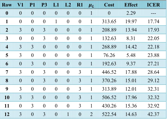
Table 3-3: Most cost-effective intervention strategies in ascending order of ICER ... 79
Table 3-4: Most effective intervention strategies in descending order of effect ... 84
Table 3-5: Optimal strategies for different levels of maximum available budget ... 85
Table 3-6: Most cost-effective intervention strategies (storng relationship among the household members) ... 88
Table 3-7: Most cost-effective intervention strategies (weak relationship among the household members) ... 90
Table 3-8: Most cost-effective intervention strategies (constant contact and reward rate) .... 92
Table 4-1: Optimization model parameters and variables for a case study motivated by vaccine allocation decisions in North Carolina ... 109
Table 4-2: Optimal Phase-I allocation for 10% and 25% for selected counties ... 123
LIST OF FIGURES
Figure 2-1: Continuous-time Markov chain associated with the SI-β model for population
size ... 30
Figure 2-2: Probability of having 1, 2, 3, and 4 infectives versus time for the stochastic model for different cases of the numerical experiment ... 45
Figure 2-3: Number of infectives versus time for the stochastic and deterministic models for different cases of the numerical experiment ... 46
Figure 2-4: Probability distribution of the epidemic duration time for different cases of the numerical experiment ... 49
Figure 2-5: Expected number of infectives versus time for the base case and all intervention policies ... 52
Figure 2-6: Probability distribution of the epidemic duration time for the base case and all intervention policies ... 53
Figure 3-1: Top 12 most cost-effective strategies on the cost-effect plane. ... 81
Figure 3-2: Efficient frontier of maximum total reward ... 86
Figure 4-1: Movement of one individual between different classes in an SEIR model ... 99
Figure 4-2: Transfer diagram for the SEIR model for population size 3 ... 100
Figure 4-3: Total expected cost for different values of (minimum Phase-I coverage), (attack rate threshold), and (percentage increase in vaccination cost in Phase-II) ... 117
Figure 4-4: Modified total expected cost for different values of (minimum Phase-I coverage), (attack rate threshold), and (percentage increase in vaccination cost in Phase-II) ... 122
Figure A-1: Weekly percentage of patient visits for ILI in flu season 2010–11 in North Carolina ... 161
Chapter 1:
Introduction
Infectious diseases have always been a threat to mankind. As an example, influenza pandemic epidemics have caused enormous societal and economic calamities. In the United States alone, the 1918 Spanish flu, the 1957 Asian flu, and the 1968 Hong Kong flu resulted in more than 500,000, 70,000 and 34,000 deaths, respectively (Longini, 2004). Further, each year there are approximately 49,000 deaths from flu-related complications in the United States from the seasonal flu according to the Centers for Disease Control and Prevention (CDC) (CDC, 2011e). According to the World Health Organization (WHO), as of August 1, 2010, 214 countries and overseas territories or communities had reported pandemic (H1N1) confirmed cases with more than 16,000 deaths (WHO, 2010). Epidemiologists warn that the next pandemic influenza could infect 33% of the population and kill millions (Gibbs, 2005). According to the CDC, it is anticipated that there will be up to $71.3–165.5 billion economic impact on the United States Economy and WHO estimates that 2–7.4 million people might die (Ekici, 2008).
The 2009 H1N1 pandemic showed that the investment the country has made in preparing for a potential pandemic has significantly improved US capabilities for a large scale infectious disease epidemic; however, it has also revealed how quickly the nation’s core public health capacity would be overwhelmed in case of a more widespread and more severe epidemic (Levi, 2009). As a matter of fact, a review of the responses to natural and man-made disasters demonstrates that during large-scale disasters, local response capacity can be quickly overwhelmed (Bravata, McDonald, Owens, 2004).
a large-scale pandemic (Bravata, McDonald, Owens, 2004). Bravata, McDonald, and Owens (2004) developed a surveillance model which suggests that although large epidemics can be relatively easy to detect using either unpooled (i.e., local) or pooled (i.e., regionalized) data analysis methods, small epidemics can be difficult to detect by either method, hence the importance of preparedness for responding to an outbreak.
In spite of the huge budget that is allocated to the health care system, there are still some inadequacies in responding to a large-scale pandemic. Decades of underfunding the public health infrastructure has stretched federal, state, and local health departments too thin to adequately respond to a large-scale pandemic (Levi, 2009). For instance, during the 2009 H1N1 pandemic, the capacity to track, investigate, and contain cases of H1N1 was hampered due to lack of resources (Levi, 2009). Therefore, it is important to spend the resources in the most effective and efficient ways to improve pandemic response capability. Therefore, not only are the effectiveness and efficiency of an intervention crucial decision factors, but also the cost of the intervention becomes an important decision factor in finding and implementing the “best” mitigation strategies, i.e., the most “cost-effective” strategies, or, the optimal level for each intervention policy.
1.1
Issues Related to Disease Spread Modeling
The issues discussed in this subsection are primarily addressed in Chapter 2, where we consider a susceptible-infective (SI) disease spread model with state-dependent contact rates and different intervention policies. Chapter 2 is mostly theoretic and functions as a theoretical basis for Chapter 3.
1.1.1 Public Adherence to Interventions
Public adherence to interventions offered by the health care system authorities is a crucial factor in the success of epidemic mitigation strategies. Some research has shown the dependency of mass prophylaxis outcomes on demand, namely, the willingness and ability of individuals in an epidemic exposure zone to access prophylactic medications either through mass dispensing sites (i.e., points of dispensing) or alternative means (US Postal Service, MedKits, etc.) (Bravata, 2006; Zaric, 2008). As a matter of fact, only a fraction of the population would opt to receive prophylactic medications such as antiviral drugs or vaccine. This partial adherence to interventions is to some extent due to possible side effects of the associated medication.
Two important factors which may affect the conformance level of the target population (Keane, 2005; Niederhauser, 2001; Rhodes, 2002; Rosenthal, 1995; Smailbegovic, 2003) are the demographic profile of the region and the quality of the information distribution regarding disease spread and interventions during an epidemic (Havicecover, 2008). Furthermore, negative experience developed during pharmaceutical campaigns in previous epidemics (Cummings, 1979; Safranek, 1991), public fear and rumors (Specter, 2009; The New York Times, 2009), and trust in the government may impact the degree of risk perception of the target population. Historically, the compliance level of health care personnel has rarely been observed to be more than 50% (Maunder, 2003; Robertson, 2004).
policies. We have represented adherence to interventions among individuals in our disease spread model in Chapter 2 by different intervention policies.
1.1.2 Public Social Behavior
After an epidemic becomes widespread, public social behavior changes and the level of precautions among individuals increases (Larson, 2007). Current disease spread models often assume a uniform rate of countermeasure dispensing once interventions begin, which may not be a realistic assumption in many cases. In Chapter 2, we propose a model which captures this change of behavior during the course of an epidemic. We relate individuals’ social behavior to the contact rate among individuals and then assume that the contact rate is a function of the number of infectives, an indicator of disease spread.
1.2
Issues Related to Optimizing Intervention Strategies
We address the issues related to the optimization of intervention strategies in Chapter 3, where we use the model developed in Chapter 2 as the theoretical basis to conduct a cost-effectiveness analysis and find the optimal level for each intervention policy for a hypothetical household. Chapter 3 is a combination of theory and application. We refer to a collection of intervention policies as an intervention strategy. For example, mass vaccination is an intervention policy while targeted vaccination of children along with isolation of infectives is an intervention strategy.
1.2.1 High Cost of Treatment
hospitals, community health centers, and primary care facilities treat large numbers of uninsured (Levi, 2009). According to the Center for Biosecurity, US hospitals could lose as much as $3.9 billion in uncompensated care and cash flow losses in a severe pandemic (Matheny, 2007). Health reform offers the opportunity to find ways to ensure all Americans would be covered during an infectious disease epidemic and that health providers would be compensated for providing care (Levi, 2009). Undoubtedly considering preventive interventions such as vaccination, isolation, and antiviral prophylaxis could result in a huge decrease in treatment costs. Furthermore, finding and implementing the most cost-effective interventions in optimal levels during an epidemic could have a large impact on reducing the treatment costs. We model this problem from a household point of view in Chapter 3 to find the most cost-effective intervention strategies and the optimal intervention strategy under a budgetary constraint.
1.2.2 Surge Capacity
The fact that surge capacity is limited makes it critically important to discover the most effective, cost-effective, and efficient intervention strategies during an epidemic. For example, it is clear that vaccine doses (if any exist) are always limited for a rare or emerging infectious disease. In addition, vaccine production may be very costly in comparison with other intervention policies such as isolation or treatment. Therefore, it is important to look for substitutable mitigation policies or a combined synergetic intervention strategy. We investigate such an intervention optimization problem in Chapter 3 from a household point of view considering the cost of each intervention policy.
1.2.3 Social Distancing Measures
As a matter of fact, WHO is now promoting social distancing as a first-order control policy (WHO, 2006). Recently, researchers at the Harvard School of Public Health have surveyed Americans who have expressed surprising willingness to engage in social distancing measures in case of a pandemic influenza (Blendon, 2009). Although social distancing and its effect on disease transmission has been separately studied in some research (Haber, 2007; Kelso, 2009), it has usually been ignored as a complementary control policy.
The 2009 H1N1 pandemic showed the challenges that communities face around decisions to close schools or work places or limit public gatherings. There are numerous ramifications for all of these actions that affect families and the economy. It is essential to consider the impact of these types of social mitigation policies and strike a balance between benefits and costs. In addition, other interventions such as vaccination and antiviral prophylaxis should be considered to minimize the cost of controlling the epidemic. We have included social distancing as a nonpharmaceutical intervention along with pharmaceutical interventions, including vaccination, antiviral prophylaxis, and treatment, to create a comprehensive framework for optimizing intervention strategies.
1.3
Issues Related to Resource Allocation
We investigate issues related to resource allocation in Chapter 4 by developing a stochastic program (SP) model to find an optimal two-phase vaccine allocation policy for geographically different regions under uncertainty in vaccination outcome.
1.3.1 Vaccination Capacity
have an adequate system in place to rapidly vaccinate all Americans; nor is there a registry in place to track the more than one vaccination (if needed) per person. When limited amounts of vaccine may be available or when it is more important to vaccinate a targeted population in advance of the rest of the community, there must be prioritization plans and people must be informed about them. For example, priority status for receiving medications or vaccinations may be used as an incentive for medical providers to increase workforce capacity (Levi, 2009). Also when vaccine doses should be allocated to geographically different regions, which might take place in more than one phase of vaccination, it is critical to allocate vaccine doses optimally so that the epidemic is mitigated with the minimum expected cost. We have investigated a two-phase vaccination policy when the outcome of the first phase is uncertain.
Another factor that might impede the nation’s ability to inoculate the entire population is the cost of vaccination. For example, according to a CDC estimate, it may cost up to $8 billion to procure 600 million doses of a novel influenza vaccine for 300 million people (if two doses per person are needed). This figure does not include needles, syringes, distribution, etc. Estimates by state and local health officials suggest that between $15 and $20 per person may be needed for administration and follow-up (Levi, 2009).
The high cost of vaccination along with its other limitations (such as availability and individual age1) raises the question “is vaccination the most cost-effective intervention?” This question may be answered by developing a model which incorporates not only vaccination effectiveness, but also its associated cost. In particular, it is important to “compare” different intervention strategies in an effort to find the most cost-effective one.
1.3.2 Timing
One very important issue for controlling an epidemic is “timing”; doing everything at its right time. From information distribution to vaccination and isolation scheduling, all need to be handled in a timely manner. Currently it seems that there is no standard timetable for different procedures that must be completed after an epidemic is detected. For example,
during the 2009 H1N1 pandemic, many private medical practitioners reported that they did not receive CDC guidance documents in a timely fashion (Levi, 2009). The impact of a delay in the start of interventions on surge severity (e.g., patient arrivals) has been studied for some particular diseases (e.g., Hupert (2009)). Also some models have been developed to estimate the effectiveness of preexposure and postexposure prophylaxes dispensing and vaccination policies in preventing large-scale epidemics (see Baccam (2007), Brookmeyer (2004), Hupert (2009), Wein (2005) for the case of anthrax). In addition, the handling of the patient loads and expected outcomes during an epidemic has been the subject of some research (e.g., see Craft (2005)).
A pandemic vaccine must be delivered to individuals as rapidly as possible. Americans receive their seasonal influenza vaccine over a period of many months, and only a fraction of the US population receives a flu vaccine annually. Health departments will need to organize (often in cooperation with the private sector) mass immunization clinics that can speed delivery of possibly as many as 100–150 million doses in a month (Levi, 2009). The importance of such efforts becomes clearer as the effect of vaccination is studied through disease spread modeling. In some cases, vaccination may occur in more than one phase due to insufficient vaccine doses at the beginning of the epidemic or to prevent unnecessary mass vaccination. We address the case of vaccine allocation to geographically different regions in two phases in Chapter 4.
phase prevents unnecessary vaccine administration. We investigate the case of two-phase vaccination in Chapter 4.
On the other hand, if prophylaxis begins too late, then it may become much harder to control the epidemic. Also if the prophylaxis is finished too soon, then it may be very costly (since it must be fully implemented in the whole community in a short time), and if it ends too late, then the number of infected people may increase and it may be difficult to control the disease. In case of limiting social contacts, if the social distancing policies end too early, then increased social mixing may cause another infection wave, which was the case in the flu epidemic of 1918 in several cities (Larson, 2007).
Time to first pill and time to last pill do not have the same importance in terms of several performance measures. For example, for a disease, such as anthrax, it has been shown that delay to campaign initiation (time to first pill) has a greater impact on casualties than campaign duration (time to last pill) (Brookmeyer, 2002, 2003, 2005; Wein, 2003) (i.e., as delay to response increases, so does variation in predicted outcomes). Nevertheless, local or state public health authorities often focus on prophylaxis campaign duration. This is understandable because the design and conduct of these campaigns are presumably directly under the purview of local or state public health authorities. In contrast, shortening the times to epidemic detection and to the decision to engage in population-wide mass prophylaxis entails a complex interplay of clinical and bio-surveillance activities that may be outside of the direct control of local public health planners (Bravata, 2002; Bravata, McDonald, Owens, 2004; Buckeridge, 2006).
1.3.3 Surveillance and Information Distribution
considered “normal.” A good syndromic surveillance system will have the capacity to alter thresholds over time to adapt to different contexts (Heymann, 2008).
It is obvious that if there is no resource2 limitation, then the best strategy is to begin interventions as the first infected case is detected and implement it in the whole community as soon as possible. But unfortunately resources are often limited as a matter of fact. Therefore, there must be a balance between benefits and costs. As a result, health care officials should try to find and implement the control strategy that would result in the “best” possible balance; or in other words, they should find and implement the most cost-effective control strategy obtained by implementing each intervention policy at its optimal level.
Although considerable effort and funding have been directed in recent years toward the development of systems and epidemic-detection algorithms, minimal evaluation of their performance in real surveillance environments has been conducted (Becker, 2003; Bravata, McDonald, Smith, 2004). The ideal evaluation approach would assess system performance by using existing epidemics of the type the system is intended to detect. However, for the majority of locations where systems are operating, essentially no previous data exist on epidemics from agents of novel infectious diseases. An alternative suggestion is to use data on seasonal epidemics as a proxy signal for evaluation (Sosin, 2003). This approach is useful but limited. Seasonal epidemics are limited in number and might differ in important ways from the type of epidemics these systems are intended to detect. Moreover, performing sensitivity analyses using real epidemic data is not usually possible (Buckeridge, 2004). Another alternative is to use simulated data for evaluation. Given the complexities of real data, evaluation should be based on real data injected with simulated epidemics as opposed to relying on fully simulated data (Sosin, 2003). To date, simulations have focused on injecting relatively simple signals with abstract characteristics into univariate time series (Goldenberg, 2002; Reis, 2003) or on creating simple and abstract spatial signals (Wong, 2002). These simulation efforts are useful for understanding the general performance characteristics of
2
detection algorithms, but they do not enable thorough evaluation of surveillance system and detection algorithm performance in realistic settings (Buckeridge, 2004)3.
Distribution of information regarding the epidemic spread as well as available interventions is critical for successful mitigation of the epidemic. The importance of information distribution becomes clearer in case of the spread of an infectious disease. In such a case, it is extremely critical to inform people of the epidemic and distribute prevention-related information throughout the population as soon as possible. In particular, the implementation of some interventions, such as self-isolation or quarantine, requires rapid information distribution and promotion in the society.
Information Technology and Decision Support Systems (IT/DSS) have the potential to help clinicians and public health officials make better decisions regarding detection, diagnosis, management, prevention, surveillance, and communication during a pandemic. However, few of these systems have been evaluated rigorously, and most were not specifically designed to address threats from an epidemic (Bravata, 2002). Since evaluation of surveillance and information support systems, such as epidemic detection and alerting systems, is critical in any effort to contain a pandemic, following a novel approach, we give an estimate of the value of these systems in Chapter 4 as the expected value of perfect information in a two-phase vaccine allocation problem.
1.3.4 Regionalization
Given the complexity and cost of training, staffing, equipping, and mobilizing an adequate pandemic response infrastructure, no single community can be expected to develop and maintain the necessary capacity for a large-scale epidemic. Instead, regionalization may benefit some pandemic preparedness and response capabilities. If there are several local responsible departments that are horizontally or vertically related to each other, then cooperative agreements and regionalized response plans are needed for effective response to
3
large-scale pandemics. Pre-event regionalized planning and asset sharing agreements among local public health agencies and hospitals may facilitate enhanced surge capacity and coordinate responses during a pandemic. Regionalization efforts have successfully expanded surge capacity for laboratory services. For example during the anthrax attacks, the Laboratory Response Network successfully provided laboratory surge capacity. Rapid communication can be difficult to achieve through interim agreements. Thus, cooperation during a pandemic may benefit from pre-event development and routine use of shared communication systems. Also in the event of a large-scale pandemic, international cooperation to detect, report, and respond may reduce associated morbidity or mortality, as it did during the SARS epidemic (Bravata, McDonald, Owens, 2004).
As a result, researchers should consider both local and multilocal approaches in their analysis and model development efforts. While the local approach deals mostly with disease spread dynamics and different mitigation strategies, the multilocal approach usually addresses the resource allocation issue. For example, a centralized stock of vaccine might have limited doses for a number of geographically different regions. We investigate this resource allocation problem in Chapter 4. We consider the cost of administering vaccine in each region and find the optimal allocation to incur the minimum total vaccination cost in all regions while ensuring epidemic containment with a predetermined probability.
1.3.5 Geographical Variations
on disease spread, etc. Accounting for these differences is key to optimizing intervention efforts in each region. We have addressed these differences in Chapter 4 in finding optimal vaccine allocation to different regions in a two-phase vaccination policy.
Policymakers recognize the need to forge relationships and coordinate preparedness planning efforts at the local, state, national, and international levels. However, there is little consensus about the optimal level of localization or regionalization for each of the resources and services that must be operationalized during a pandemic response (Bravata, McDonald, Owens, 2004). In the United States, special populations including children, the elderly, the disabled and pregnant women account for about 134 million people (Hetzel, 2003; National Center for Health Statistics, 2003; US Census Bureau, 2003a; 2003b). Thus, emergency preparedness planning requires consideration of these special populations. However, there is little evidence that specifically addresses variations in regionalized responses on the basis of geography, population, or public-private cooperation (Bravata, McDonald, Owens, 2004).
For the purpose of examining policy-level decisions about public health emergency response, using a defined target population makes practical sense because policy makers ultimately may want to ensure that planning encompasses their specific jurisdictions, for which the size is known. In addition, for many diseases, including H1N1, the estimates of some principal disease parameters, such as the basic reproduction number4, vary from one country to another. Furthermore, using simple population exposure estimates may allow more transparent planning for worst-case scenarios that involve entire target populations than using estimates which are modified by incidental effects such as atmospheric conditions (Hupert, 2009). Therefore, any realistic modeling approach should customize the model parameters according to the specifications of a target population.
4
1.3.6 Response Supply Chain
In a rather large-scale pandemic, having an effective and efficient response supply chain is vital. In case of an infectious disease epidemic, supply chain related issues include, but are not limited to, delivering prophylaxis and vaccine doses to the target population at the scheduled time, delivering treatment services to the infective individuals, and providing adequate facilities for hospitalization and quarantine. If the supply chain capacity does not allow for mass interventions, then an alternative is to implement interventions in more than one phase. We have investigated the case of vaccine allocation to different regions in two phases in Chapter 4.
1.4
Review of Epidemic Modeling
Mathematical models have been widely used as important tools in analyzing the spread and control of infectious diseases. Mathematical models and computer simulations are useful experimental tools for examining theories, determining sensitivities to changes in parameter values, assessing quantitative conjectures, estimating key parameters from data, and finding the answer to specific questions (Hethcote, 2000). Epidemiological modeling has also been used to design and analyze epidemiological surveys, identify critical data that should be collected, detect trends, make general predictions, and estimate the uncertainty in forecasts (Hethcote, 1989; 1992).
Since the middle of the 20th century, mathematical epidemiology demonstrated an exponential growth. A review of the literature proves this rapid growth (Becker, 1978; Castillo-Chavez, 1990; Dietz, 1967, 1985, 1988a; Hethcote, 1981, 1989, 1994; Wickwire, 1977). In addition, several models were developed for particular diseases such as measles, rubella, chicken pox, whooping cough, diphtheria, smallpox, malaria, onchocerciasis, filariasis, rabies, gonorrhea, herpes, syphilis, and HIV/AIDS (Hethcote, 2000). For example, see Ferguson (2003) for a review of spread models for smallpox and see Lipsitch (2003) and Riley (2003) for SARS. Furthermore, several books have been written on epidemiological modeling (Anderson, 1982a, 1982b; Bailey, 1982; Bartlett, 1960; Becker, 1989; Busenberg and Cooke, 1993a; Capasso, 1993; Cliff, 1988; Frauenthal, 1980; Gabriel, 1990; Grenfell, 1995; Hethcote, 1984; Isham, 1996; Kranz, 1990; Lauwerier, 1981; Nasell, 1985; Scott, 1994; Vanderplank, 1963; Waltman, 1974).
A special class of epidemiological models consists of compartmental models. It is quite common to use compartmental models to represent the spread of an infectious disease. The foundations of the approach to epidemiology based on compartmental models were laid by public health physicians such as R.A. Ross, W.H. Hamer, A.G. McKendrick and other researchers such as W.O. Kermack between 1900 and 1935 (Brauer, 2008).
Some of the efforts in modeling epidemics have focused on developing data-based statistical models to examine the statistical aspects of the epidemic. The main goal of such models is to estimate epidemiological parameters primarily using likelihood- or regression-based approaches (Cauchemez, 2004; Longini, 1982; 1986). On the other hand, some researchers have focused on the virus spread dynamics and transitions between disease phases. These efforts resulted in several mathematical models which are usually represented in a system of differential equations (Arino, 2006; Cahill, 2006; Fraser, 2004; Larson, 2007; Wu, 2007). Also there are some mathematical models which use random graphs (Carrat, 2006) and difference equations (Grais, 2003; Rvachev, 1985) to model an epidemic.
In addition to statistical and mathematical models, simulation-based models5 have been developed to model disease spread and also examine the impacts of different interventions, including vaccination, antiviral prophylaxis, isolation, and treatment (Das, 2008; Ferguson, 2005, 2006; Germann, 2006; Glass, 2006; Longini, 2004; Patel, 2005; Wu, 2006). Some of these models integrate different types of interventions seeking synergetic strategies. A good example of such models is the network model of MIDAS (Models of Infectious Diseases Agent Study), which used three independent simulation models to examine different interventions in 2006–07 (Halloran, 2008). These models were used to simulate large-scale pandemic influenza spread for rural areas of Asia (Ferguson, 2005; Longini, 2005), the United States, and the United Kingdom (Ferguson, 2006; Germann, 2006), and the city of Chicago (Eubank, 2004). The Institute Of Medicine (IOM) has published the major findings of the MIDAS group and other institutions (Atkinson, 2008; Glass, 2006) as recommendations regarding mitigation of pandemic influenza at the local level in a report entitled “Modeling Community Containment for Pandemic Influenza” (IOM, 2006).
Some of the guidelines and research have focused on specific interventions, including antiviral prophylaxis and treatment (CDC, 2009c, 2009e), vaccination (CDC, 2009a; Pasteur, 2009; Washington State Department of Health, 2009), and isolation (CDC, 2009b; Ekici,
5
These simulation models include both agent‐based models (which track each individual) and event‐based
2008; Haber, 2007; Kelso, 2009). Furthermore, “cost” is a fairly recently considered factor in assessing different interventions. Also as stated previously, social distancing, which may be very effective in mitigating the epidemic, has rarely been included in disease spread models. We have incorporated both cost and social distancing measures in our epidemic models, in addition to vaccination, antiviral prophylaxis, and treatment (in the analytical epidemic model), which together create a comprehensive framework for disease spread and optimization of interventions. In addition, the decision makers in our model are members of a household (see Chapter 3) as opposed to public health officials or individuals who are the main decision makers in most of the current research on optimizing intervention strategies. Finally we have used a combination of analytical and simulation methods throughout this dissertation to take advantage of both approaches.
1.5
Research Question and Methodology
During an epidemic, the most important task for health care officials is to identify and implement the most effective interventions for controlling the epidemic. However, there are always limitations associated with the implementation of counter measures. For example, after a new influenza virus subtype is identified, it may take up to six months to produce a potent vaccine in sufficient quantity (Aunins, 2000; Fedson, 2003). Even if the emerging virus belongs to a known subtype, available vaccine doses may not be adequate for the entire population; nor may be antiviral drugs. In addition, available budget is always an inevitable constraint and therefore it should be spent on the most effective interventions. These issues bring another important decision factor into the picture: the “cost” of different interventions. Considering both “effectiveness” and “cost” of an intervention leads us to the “cost-effectiveness” analysis, which is currently widely used to compare different mitigation strategies and find the “best” one.
concentrate on susceptible individuals. Vaccination reduces the number of susceptibles in the case of a perfect vaccine, or the susceptibility of vaccinated individuals in the case of an imperfect vaccine. Antiviral prophylaxis reduces the susceptibility of individuals similar to an imperfect vaccine. On the other hand, some interventions target infective individuals. Isolation among infectives reduces the number of infectives who contribute to disease spread. Treatment reduces the infectivity of infective individuals or removes them from the infective population if treatment occurs in a health care setting or can be assumed perfect.
There is a cost associated with each of these intervention policies. The question is “Which one is more effective and less costly?” In other words, “Which one is more cost-effective?” or “If there is an optimal combination of different intervention policies, what is the optimal combination?” Another research question addressed in this research concerns resource allocation in the case of limited vaccine doses which should be allocated to geographically different regions in two phases: “What is the optimal allocation which results in the minimum expected total cost?” We have used the modeling approach to answer these questions.
isolation, and treatment considering both full and partial adherence to interventions among individuals.
The model is applicable to any infectious disease in which any individual can be considered either susceptible or infective (with negligible recovery and death rate in the horizon under study). HIV is an example of such diseases. Also if the disease is very contagious or if a relatively short horizon is considered, then the model can be applied to the early stage of any infectious disease with an insignificant latent period at the epidemic.
In Chapter 3, we identify optimal intervention strategies in case of an epidemic. We consider an affected household (a household with one initial infective member) and model the effect of different intervention policies, which involve vaccination, antiviral prophylaxis, isolation, and treatment, on disease spread using a variation of Kermack-McKendrick models. Both full and partial adherence to interventions are considered. An implementation cost is assumed for each intervention policy. We refer to a collection of intervention policies as an intervention strategy. A reward is associated with susceptible members who remain uninfected. We define the effect of the implemented strategy as the total reward earned by all members over the time horizon. We evaluate the cost-effectiveness of strategies and identify the most cost-effective intervention strategies. In addition, we incorporate a budgetary constraint for the household and find the efficient frontier for the total reward over different upper bounds on the household budget allocated for intervention.
reduces to a linear program with a similar size to that of the first stage problem. We construct test cases motivated by vaccine planning in North Carolina. We find the optimal vaccine allocation and estimate the value of the stochastic solution and the expected value of perfect information. We also propose and test some easy to implement heuristics for vaccine allocation.
Chapter 2:
Analytic Solution of the Stochastic
Susceptible-Infective Disease Spread Model with
State-Dependent Contact Rates and Different Intervention
Policies
Abstract
We consider the susceptible-infective (SI) epidemiological model, a variant of the Kermack-McKendrick models, and let the contact rate be a function of the number of infectives, an indicator of disease spread during the course of the epidemic. We represent the resultant model as a continuous-time Markov chain. The result is a pure death (or birth) process with state-dependent rates, for which we find the probability distribution of the associated Markov chain by solving the Kolmogorov forward equations. This model is used to find the analytic solution of the SI model as well as the distribution of the epidemic duration. We use the maximum likelihood method to estimate contact rates based on observations of interinfection time intervals. We compare the stochastic model to the corresponding deterministic models through a numerical experiment. We also incorporate different intervention policies for vaccination, antiviral prophylaxis, isolation, and treatment considering both full and partial adherence to interventions among individuals.
2.1
Introduction
Ordinary differential equations (ODEs) are the basis for many population models in epidemiology. The Kermack-McKendrick model (Kermack, 1927) was one of the first models developed to simulate the number of infectives associated with diseases such as bubonic plague (London 1665–66, Bombay 1906) and cholera (London 1865). Many variations of the original Kermack-McKendrick model have been developed. Generalizations of this model are sometimes referred to as SEIRS (susceptible, exposed, infective, and recovered) models. We will refer to the Kermack-McKendrick model and its variations as KM models. Hethcote (1976) investigated a variety of KM models including the SI, SIS, and SIR variations.
In the case of a highly contagious disease which spreads quickly or in the short term, especially at the beginning of an epidemic when the effects of recovery and death can be ignored, the SI model is quite appropriate for characterizing disease dynamics (Bai, 2007; Zhou, Liu, 2006). Under these circumstances, the population can be categorized into two compartments (or epidemiological classes) at each point of time, susceptible (S) and infective (I). The SI model also has applications in technological communication networks (Krause, 2006), broadcasting processes (Gupta, 2000), email system services (e.g., Google when membership was only by invitation), and network marketing processes (Kim, 2006).
equilibrium points, conduct sensitivity analysis on different model parameters, and find the distribution of the epidemic duration.
In KM models, it is assumed that the contact rate, which is a reflection of people’s social behavior regarding disease spread, is constant during the course of the epidemic. However, people’s social behavior changes as society copes with an epidemic (Larson, 2007). Therefore it is more realistic to model contact rate as a function of the number of infectives, because the number of infectives is an indicator of disease spread and its threat for susceptible individuals.
Homogeneity of the population is a basic assumption of the (deterministic differential equation) KM models, which might be valid for small populations. However, in a small population, stochastic effects play an important role in the dynamics of disease spread. Even if we are only interested in mean values, we still need to take into account the stochastic effects because stochastic means are not equal to their corresponding deterministic values for nonlinear epidemic processes (Bailey, 1957).
In this research, we formulate a generalization of the SI model with state-dependent contact rates, denoted by the SI-β model, as a continuous-time Markov chain (CTMC). We solve the Kolmogorov forward equations for this CTMC and find the probability distribution for the state of the system as an explicit function of time. We use the state probability distribution to find the analytic solution of the SI-β model as well as the distribution of the epidemic duration. Lastly we incorporate different intervention policies including vaccination, antiviral prophylaxis, isolation, and treatment into the SI-β model by relating the intervention effects to the contact rate during the course of the epidemic. We consider both full and partial adherence to interventions among individuals.
on the interinfection time intervals. We consider a household size of four individuals and compare the stochastic solution of the SI-β model with the deterministic solution of the SI model. In Section 2.5, we incorporate different intervention policies into the model. We conclude this chapter in Section 2.6 by summarizing our findings and suggesting some directions for future research.
2.2
Literature Review
Literature related to solutions of KM models fall in two general categories: epidemiology and nonepidemiology based models. First we briefly review the literature in the first category, which is not as developed as the second category.
Newman (2002) used a network approach to analyze the SIR model for a fixed infectious time and fixed probability of transmission between all pairs of individuals. He showed that the SIR model can be solved exactly for a wide variety of networks. He has also solved cases in which times and probabilities are nonuniform and correlated. Gani (1965) considered the differential equations for the SIR model with constant population size. He outlined a mathematical method for solving the partial differential equation which the associated probability generating function satisfies. However, the mathematics involved are so complicated, limiting its application to small population sizes of at most three individuals. Gart (1968) considered an SI model with constant population size and two types of susceptibles having very different infection rates. He derived the exact solution in an implicit form and also an approximation to the solution which permits simple estimates of the infection rates.
(Laubenbacher, 2004) to find discrete approximations for the associated KM model. Allen and Burgin (2000) analyzed the dynamics of the deterministic and stochastic discrete-time SIS and SIR models with constant population size and the SIS model with variable population size. They also examined the expected duration of the epidemic numerically. Castillo-Chavez and Yakubu (2001) considered the discrete-time SIS model in a population with complex chaotic dynamics. They assumed various levels of complexity to examine the effect of density-dependent population dynamics on disease dynamics. They considered a variable (state-dependent) infection probability in their discrete-time model.
Even in the absence of uncertainty, traditional numerical methods, such as Euler’s method or Runge-Kutta schemes, only approximate the ODE system solution as truncation errors from both function approximation and machine arithmetic are present. When there is uncertainty in the initial conditions, traditional methods cannot account rigorously for the uncertainties. Therefore there have been efforts to find verified (i.e., mathematically and computationally guaranteed) solutions of such systems of ODEs. For example, Enszer and Stadtherr (2010) considered continuous epidemiological models that are systems of ODEs and formulated as initial value problems (IVPs). They used interval methods (also called validated or verified methods) to find rigorous bounds on the solution of these systems of ODEs. These solutions are particularly applicable to systems that involve uncertainty in initial conditions or model parameters.
equations considerably due to absence of repeated roots. Moreover, Bailey provided a solution when the total population size (except for the one initial infective individual) is even. Severo (1967) gave the solution to a special form of triangular ODE systems and used it to find the analytic solution to the stochastic SI and SIR models of Bailey (1957). His work is similar to ours in the sense that he considered a general probabilistic initial condition. However, similar to Bailey’s work, he assumed a constant contact rate. In some research (Ball, 1993; Gleissner, 1988; O'Neill, 1997; Severo, 1969a) special functional forms for the infection (and recovery) rate are considered, but general rates are missing.
Billard et al. (1979), following a different approach, considered the SI model with the initial condition of one infective individual. They represented the distribution of the number of infectives as a convolution of exponential waiting times to find the analytic solution for the SI model with a constant contact rate as opposed to the more general state-dependent contact rates considered in our research.
In the second category of related literature, which consists of nonepidemiologic models, there are two streams of literature: birth and death processes (BDPs) and right-shift processes, a class of Markov processes with multidimensional finite state space on which the infinitesimal transition movement is a shifting of one unit from one coordinate to another coordinate to its right (Severo, 1969c). KM models with more than two classes can be represented as right-shift processes.
triangular system, which can be solved by the method described in Severo (1969b). Billard (1981) gave the analytic solution for a bounded two-dimensional birth and death process (2-BDP) where the transition rates are time-independent functions of the population state. Billard’s approach was based on the combined techniques of Severo (1969b, 1969c), where she worked directly with the Chapman-Kolmogorov equations. Parthasarathy and Sudhesh (2006) presented a power series expression in closed form for the transient probabilities of a state-dependent 1-BDP. They transformed the underlying forward Kolmogorov differential-difference equations into a set of linear algebraic equations by employing Laplace transforms, and then used continued fractions to derive the transient probabilities. Brandwajn (1979) developed a seminumerical iterative approach to the solution of the balance equations of a finite 2-BDP. His method is seminumerical in that it used the formal knowledge of the stationary probability distribution of one variable, and the iteration is applied to the conditional probabilities of the second variable given the first one.
Some of the models in both categories only give approximate solutions to KM models. In most of the models that produce the exact solution, the complexity of the mathematics limits the application to small population sizes. In addition, some of these models only provide the exact solution for special cases, under limiting assumptions, or in an implicit form. Also most epidemic models developed in the literature assume a constant contact rate and a deterministic initial condition. Furthermore, partial adherence to interventions is usually ignored in the current literature. In comparison with the existing literature, our model gives the exact solution for the SI model with state-dependent contact rates and with a general probabilistic initial condition in an explicit form. We also incorporate different interventions considering both full and partial adherence to interventions.
2.3
Representing the SI-
β
Model as a CTMC
short that births and deaths could be ignored, which is the case for a highly contagious disease. We denote the susceptible and infective population at time by and (or simply and ), respectively, and the total population size by . Because there are no vital rates we have a closed population, that is the total population size is constant and we have
for all times .
If we denote the average number of contacts of one individual per unit time by , and the probability of disease transmission when a susceptible makes a contact with an infective by , then the average number of effective contacts (i.e. contacts sufficient for disease transmission) of one individual per unit time would be . If a susceptible makes a contact at time , with probability / 1 this contact is with an infective, and therefore, / 1 gives the average number of effective contacts of one susceptible with an infective per unit time at time . Thus the average number of effective contacts of all susceptibles with infectives per unit time, or the horizontal incidence (the rate at which susceptibles become infected) at time is / 1 . In the literature of KM models, it has become a convention to use in the denominator instead of 1 because a large population size is usually being considered. In this case the horizontal incidence is given by
(2-1) and is known as the standard incidence (Hethcote, 2000). Using the standard incidence in
(2-1) slightly changes the interpretation of , particularly in a small population. More precisely, if is the true effective contact rate, the parameter should be set to / 1 in a small population to be able to use the standard incidence given in (2-1). Note that the factor
1/ or 1/ 1 can also be absorbed into the definition of the parameter (e.g. in Bailey (1957)). In this chapter, and in Chapter 3, we will use (2-1) to calculate the infection rate to be consistent with the convention and for notational simplicity, refer to the parameter as the “effective contact rate”, or the “contact rate”.
infectives. Note that a state-dependent contact rate indeed represents the change in the susceptibles’ behavior with respect to disease spread. The function is typically nonincreasing in as a result of a higher level of precaution (e.g., washing hands more frequently) when the epidemic is widespread (however, this is not a requirement in our model).
If , denotes the state of the system at time , the state space would be
, ∈ | , 0 , 1,1 , 2,2 , … , 1, 1 , 0, ,
where denotes the set of nonnegative integers. The size of the state space is given by
| | 1
1 , (2-2)
where denotes the number of epidemiological classes; therefore 2 for the SI-β model and we have | | 1. Note that formula (2-2) gives the number of ways to sum non-negative integer numbers to get the positive integer . For example, in an SI-β model with 20 individuals, there would be 21 states in according to formula (2-2). The associated stochastic process is a right-shift process in which the only state transition occurs if one individual moves from compartment S to compartment I with the following transfer rates obtained from (2-1) for the original state , ,
, , 1, 1 , 0, (2-3a)
, 0 , otherwise. (2-3b)
If we define the stochastic process , then is a pure death process, which is a 1-BDP. Alternatively, we may define the stochastic process to obtain a pure birth process. The associated CTMC, which we will refer to as CTMC-SI-β, for population size is shown in Figure 2-1.
Note that we have eliminated the state , 0 in CTMC-SI-β, because without any infectives there would be no dynamics.
2.4
Analytic Solution of the SI-
β
model
In this section, we derive the Kolmogorov forward equations for CTMC-SI-β. The fact that the SI-β model can be represented as a pure death (or pure birth) process results in a triangular structure in the linear ODE system obtained from the Kolmogorov forward equations. This makes it possible to solve the equations iteratively and find the analytic solution for the SI-β model. The details are as follows.
We refer to state , as state . Let 1,2, … , 1 be the set of the possible number of infectives before the epidemic ends with the infection of the th individual. Let , 1,2, … , , be a row vector denoting the state probability distribution, where 0 denotes the probability that CTMC-SI-β is in state at time and ∑ 1 for all 0. The initial probability distribution is 0 0 ,
1,2, … , . Therefore the expected value of the initial number of infectives would be
0 ∑ 0 . Also let , , 1,2, … , be the transition
rate matrix so that denotes the rate at which CTMC-SI-β makes a transition from state into state . Then from (2-3) we have
, 1, ,
, , ,
0, ,
(2-4)
for , 1,2, … , .
We derive the Kolmogorov forward equations for CTMC-SI-β using (2-4). We drop for simplicity of notation. If we denote the column of by , then the Kolmogorov forward equations can be represented as follows,
Therefore for CTMC-SI-β we obtain from (2-5) the following triangular linear ODE system,
,
, 2,3, … , 1,
, (2-6)
where , ∈ , represents the horizontal incidence when there are infectives. Note that the right side of the equations in (2-6) sum to zero, verifying
∑ ∑ 0 1 , 0. (2-7)
We find the analytic solution of system (2-6) using the following lemma.
Lemma 2-1: If is a continuously differentiable real-valued function for 0 which satisfies the differential equation
∑ , (2-8)
( being a nonnegative integer) with the boundary condition 0 and if , 1,2, … , , then
∑ ∑ . (2-9)
Proof:
By taking the derivative of both sides of (2-9) with respect to , we have
∑ ∑ ∑ ∑
∑ ∑ .
Also satisfies the boundary condition 0 . Therefore given by (2-9) is a solution of differential equation (2-8), uniqueness of which follows from the uniqueness theorem for ODEs.∎
Proposition 2-1: If , ∈ satisfy
, 2,3, … , 1, 1,2, … , 1, (2-10)
then the solution of system (2-6) is
,
∑ , 2,3, … , 1,
1 ∑ ,
(2-11)
where
0 , 1,
0 ∑ , 2,3, … , 1,
, , 2,3, … , 1, 1,2, … , 1.
(2-12)
Proof:
Applying Lemma 2-1 (with 0 and ) to the first equation in (2-6), , implies 0 . Therefore 0 as given by (2-12). Substituting in the second equation in (2-6) implies . Condition (2-10) implies
, 2,3, … , 1, 1,2, … , 1. Therefore and Lemma 2-1 (with
1 and ) implies 0 . Therefore
and 0 , as given by (2-12). Other coefficients are calculated by applying Lemma 2-1 to system (2-6) iteratively in a similar way. The associated coefficients for the case 4 are calculated in Subsection 2.4.3.∎
If 0, ∈ , then there is only one absorbing state in CTMC-SI-β, which is state , and all other states are transient, since from (2-11) we have
lim → 0 , ∈ , (2-13a)
lim → 1, (2-13b)
The analytical solution of the SI-β model as the stochastic mean of CTMC-SI-β is
∑ , (2-14a)
For any population size , the recursive equations in (2-12) may be used to obtain coefficients , which are used in (2-11) to calculate , 1,2, … , . Finally the exact solution of the SI-β model can be calculated using (2-14).
There are two points which should be noted regarding Proposition 2-1. The first is that ’s are not a function of as shown in Proposition 2-1. This is due to the fact that there are no dynamics if the entire population is already infected. The second is that condition (2-10) is not practically binding. If condition (2-(2-10) is not satisfied, then the values of the nonconforming ’s could be perturbed by some 0 to satisfy condition (2-10). This approach to satisfy condition (2-10) is illustrated in Subsection 2.4.3. A special case for which we can still find the exact value of , 1,2, … , even if condition (2-10) is violated is when both sides of (2-10) are equal to zero for some ∈ 2,3, … , 1 and
∈ 1,2, … , 1 . Note that if condition (2-10) is violated for a pair and , then we cannot
calculate using Proposition 2-1 because the denominator would be equal to zero in calculating . Let min | 0 0, 1,2, … , which implies 0, ∈
1,2, … , 1 , 0. If condition (2-10) is violated with both sides equal to zero for some
∈ 2,3, … , 1 , we simply set 0, 0 and calculate other probabilities using
(2-11). If instead condition (2-10) is violated with both sides equal to zero for some ∈
, 1, … , 1 , we need the following assumption to find the exact value of ,
1,2, … , .
Assumption 2-1: If 0 then 1 0 for ∈ , 1, … , 2 .
Note that this assumption is consistent with the fact that, as we mentioned previously, is typically nonincreasing in as a result of higher level of precautions among individuals when the disease is widespread. Further, the case of 0 indeed represents a strong counter measure to contain the epidemic, e.g., quarantine of infectives enforced by health care authorities, which reasonably must be also implemented where there are 1
Assumption 2-1ʹ: If condition (2-10) is violated with both sides equal to zero for a pair
∈ , 1, … , 1 and ∈ 1,2, … , 1 , then 0 for some such that
∈ , 1, … , 1 where max ∈ | 0 0, .
Under Assumption 2-1 (or Assumption 2-1ʹ), it is only possible to have infectives at any
0 if there are initially infectives, that is, event 0 occurs. Therefore in this case we set Pr 0 0 , 0. We do this for all pairs ∈ , 1, … , 1 and ∈ 1,2, … , 1 which violate condition (2-10) with both sides equal to zero and then calculate the other probabilities using (2-11).
It seems intuitive that if the contact rates are reduced (e.g., due to an intervention), then the expected number of infectives at any time 0 should decrease. This turns out to be the case as formally stated in Theorem 2-1. First we need the following definitions and the subsequent propositions.
Definition 2-1: A state ∈ is an impossible state if 0 for all 0, otherwise the state is a possible state.
Proposition 2-2: State is an impossible state if and only if, (a) 0 0, and
(b) 0 for some ∈ , 1, … , 1 where max ∈ | 0 0, .
Proof:
Assume is an impossible state. Then (a) follows directly from the definition of an impossible state. The interinfection time interval when there are infectives is exponentially distributed with rate (see Subsection 2.4.2). If (b) does not hold then 0, ∈
, 1, … , 1 . Therefore it follows by a simple conditioning process on the state of
and (b) hold. It follows from (a) that 0 0. Therefore the only way CTMC-SI-β can reach state is through states , 1, … , 1. But 0 implies 0, and therefore, state is an absorbing state making it impossible to reach state . Therefore 0 for all
0 and state is an impossible state.∎
Proposition 2-3: If is a possible state, then 0 for all 0.
Proof:
Since is a possible state there exists ̅ 0 such that ̅ 0. The interinfection time interval when there are infectives is exponentially distributed with rate (see Subsection 2.4.2). Therefore conditioning on the current state of CTMC-SI-β at ̅ we obtain ̿
0 for any ̿ ̅. If 0 0, the proof is complete by setting ̅ 0. Assume 0 0. Since is a possible state, it is not an impossible state by definition and therefore since part (a) of Proposition 2-2 holds, part (b) does not hold. Therefore, as in the proof of Proposition 2-2, it follows by a simple conditioning process on the state of CTMC-SI-β at 0 that
0 for all 0.∎
Theorem 2-1: If , , ∈ are two contact rate vectors which satisfy
, ∈ , (2-15)
then,
for all 0, (2-16)
Proof:
Condition (2-15) implies , ∈ , where is the counterpart of for the contact
rate vector . Let ∑ and ∑ , where is the
counterpart of for the contact rate vector . We have
∑ ∑ ∑
∑ 1 ∑ ∑ , (2-17a)
∑ ∑ ∑
∑ 1 ∑ ∑ . (2-17b)
where ∑ ∑ ≡ 0 if 1. Therefore (2-16) is equivalent to
∑ ∑ for all 0; and if we show
, ∈ for all 0, (2-18)
with strict inequality for at least one ∈ if we have strict inequality in (2-15) for at least one possible state,then Theorem 2-1 is proven. First we show (2-18) holds by induction. For
1, we have 0 and 0 . Since
0 0 and 0, we have for all 0. Now we show if
(2-18) holds for ∈ 1,2, … , 2 then it must also hold for 1 by contradiction. Assume (2-18) holds for ∈ 1,2, … , 2 but it does not hold for 1. By taking the derivatives of and with respect to time, from (2-6) we have,
0, (2-19a)
0. (2-19b)
Consider the function . Since (2-18) does not hold for 1 by assumption, there must be a point 0 such that 0. Let max ∈
0, | 0 . Since 0 0 ∑ 0 , we have 0 0, and