DOI: 10.1534/genetics.105.047472
Inferring Population Parameters From Single-Feature Polymorphism Data
Rong Jiang,* Paul Marjoram,
†Justin O. Borevitz
‡and Simon Tavare´*
,§,1*Molecular and Computational Biology Program, University of Southern California, Los Angeles, California 90089,†Department of Preventive Medicine, Keck School of Medicine, University of Southern California, Los Angeles, California 90089,‡Department of Ecology and Evolution,
University of Chicago, Chicago, Illinois 60637 and§Department of Oncology, University of Cambridge, Cambridge CB2 2XZ, England Manuscript received June 29, 2005
Accepted for publication May 3, 2006
ABSTRACT
This article is concerned with a statistical modeling procedure to call single-feature polymorphisms from microarray experiments. We use this new type of polymorphism data to estimate the mutation and recombination parameters in a population. The mutation parameter can be estimated via the number of single-feature polymorphisms called in the sample. For the recombination parameter, a two-feature sampling distribution is derived in a way analogous to that for the two-locus sampling distribution with SNP data. The approximate-likelihood approach using the two-feature sampling distribution is examined and found to work well. A coalescent simulation study is used to investigate the accuracy and robustness of our method. Our approach allows the utilization of single-feature polymorphism data for inference in population genetics.
N
ATURAL variation is of great interest to a variety of disciplines, such as evolutionary biology, plant and animal breeding, human genetics, and population genetics. For example, it enables us to study the effects of genetic forces, infer population history, and under-stand the genetic basis of complex traits. There are several types of genetic data available to study natural variation, including restriction fragment length poly-morphisms (RFLPs), microsatellites, and single nucle-otide polymorphisms (SNPs).Microarrays, a high-throughput technology for ge-nomic DNA/RNA hybridization, play a key role in functional genomics. Two major applications of DNA microarrays are expression analysis and genotyping. With the development of microarray technology and design, more accurate and robust statistical methods are needed to analyze the massive amount of data pro-duced. Detailed examples may be found in Parmigiani
et al. (2003) and Speed(2003), for example.
As a model plant, Arabidopsis thaliana has been extensively investigated in areas such as plant physiology and crop breeding. Borevitzet al. (2003) used Affyme-trix arrays to detect the genomic DNA signal in A. thaliana and conducted genomewide studies such as gene clustering, deletion identification, and quantita-tive trait loci (QTL) mapping. Along with new develop-ments of array design, otherA. thalianaaccessions have been studied. Wolynet al. (2004) studied the variation
between the accession Kas and the reference Col to map the light response QTL. Werneret al. (2005) studied two accessions, Bur-0 and Lz-0, for F2extreme array QTL mapping.
The scaled mutation parameter u and the scaled recombination parameter r are important quantities in population genetics studies. Watterson(1975) derived a point estimator of u based on the number of seg-regating sites, assuming the infinitely many sites muta-tion model. For r the situation is more complex, but there are several approaches using SNP data, for ex-ample, rejection-based methods using summary statis-tics (Wall2000) and approximate-likelihood methods (Hudson 2001; Liand Stephens 2003; McVeanet al. 2004).
In this study, we develop methods to model and an-alyze single-feature polymorphism (SFP) data. Our focus is on estimatinguandr, which will help us explore and utilize this new type of polymorphism data in more general settings. First we revisit the microarray experi-ment in Borevitz et al. (2003) and describe in detail how we model the statistical procedure to call features. We show how the number of features called can be used to estimate u. An approximate-likelihood approach is proposed to estimate r by deriving the two-feature sampling distribution by analogy with the two-locus sampling distribution in Hudson(2001). We assess the accuracy of this estimator using coalescent simulations. Finally, we investigate statistical properties of our maximum-likelihood estimator of r and check the robustness of our approach by varying demographic parameters. We also discuss how much information is lost in SFP data compared with SNP data.
1Corresponding author:Molecular and Computational Biology Program,
University of Southern California, 835 W. 37th St., SHS172, Los Angeles, CA 90089-1340. E-mail: [email protected]
MODELING
Motivation: Borevitz et al. (2003) studied allelic variation in ecotypes ofA. thaliana. DNA was prepared independently from three Col and three Lerplants and hybridized to six Affymetrix expression arrays. We refer to Col as the reference type and Ler as the accession. The arrays were set up to match the reference genome sequence. After the arrays were scanned, the mean intensity of each probe was spatially corrected, quantile normalized, and analyzed by the SAM method (Tusher
et al. 2001). A probe was called as an SFP if its hybrid-ization intensity was detected as being significantly dif-ferent from that for the corresponding reference probe. An illustration of SFP calling between two strains is given in Figure 1. In Borevitzet al. (2003), 3806 SFPs were called out of 92,924 unique probes and these were used later for detecting potential deletions and for bulk segregant analysis.
Although comparing accessions one at a time against the reference provides only pairwise diversity, we can combine these pairwise comparisons and produce SFP data across multiple accessions in a similar way to that in which we call segregating sites: a feature is called poly-morphic if there is at least one accession probe at this position whose hybridization intensity is called statisti-cally significantly different from that of the reference probe. We can model this scheme exactly in our sim-ulations. At this time, 19 accessions are examined in the Borevitz lab and the SFP data from this group of accessions plus the reference strain serve as the basis for our inference of population history forA. thaliana.
We now revisit the procedure for obtaining the SFP data. There are two main steps in the microarray experiments: measuring hybridization intensity for each probe and detecting significant differences of hybrid-ization intensity with respect to the reference, as illustrated in Figure 1. The latter is a purely statistical procedure and we do not attempt to model it at the sequence level. Nevertheless, we use independent se-quence confirmation of called SFPs to quantify this step and include it in our simulations. Below, we describe in detail how to model the SFP-calling procedure in coalescent simulations.
The coalescent: Pioneered by Kingman (1982), Hudson(1983), and Tajima(1983), coalescent theory continues to prove a useful model for studying neutral population history. In particular, fast and efficient coalescent simulations help us to test the fit of different models to data, especially when analytical results are hard to obtain. For reviews of coalescent theory and related inference methods, see Nordborg (2001), for example. We use the coalescent to model the genealogy of the accessions and the reference.
The issue of sample size and selection of the reference sample requires some thought in coalescent simula-tions. Suppose that 19 accessions plus the reference (Col) are in the microarray experiment. We simulate only one haplotype for each ecotype (either accession or reference), since A. thaliana is highly selfing and therefore its genome is essentially homozygous (see Nordborg et al. 2005 for a discussion of this issue). Therefore, we set the sample size as 20 when we deal with 20 different ecotypes. Moreover, the reference is chosen randomly among the simulated haplotypes, since the strain Col is chosen as the reference merely because it was the first strain completely sequenced. In other words, there is nothing special about this strain compared with other strains. Last, the sample of hap-lotypes is simulated using the ms program (Hudson2002) and then postprocessed to obtain SFP data. We simulate samples without population structure.
SFP comparison phase: For the simulated data, we are able to measure the sequence polymorphism at each probe position for every accession compared to the reference, instead of needing to measure hybridization intensity in microarray experiments. For simplicity, we restrict our mutation model to consider only single-nucleotide polymorphisms. There are several types of sequence polymorphism within a 25-bp probe when comparing an accession to the reference. We classify them as follows: no difference, one-SNP difference, and more-than-one-SNP difference. Noting that the chance of having more than one SNP within a 25-bp probe is rather small, we take it as an assumption later and categorize the sequence polymorphism as either ‘‘no difference’’ or ‘‘one-SNP difference.’’
In simulations, each accession is compared with the reference at every probe position. If in fact there is more than one SNP in a given probe, it is treated as having a one-SNP difference. Consequently, every probe of each accession is labeled 0 (no difference) or 1 (one-SNP difference) after comparisons.
SFP-calling phase: In microarray experiments, high or low hybridization intensities are called significant by a prespecified statistical procedure, involving results from multiple hypothesis testing. It is not easy to model this step without taking into account the array setup and the distribution of test statistics. On the other hand, we can characterize the statistical procedure by summarizing the four types of possible outcome: true positives, true
Figure1.—Calling an SFP between the reference Col and
negatives, false positives, and false negatives. Borevitz
et al. (2003) confirmed the SFPs called by comparing available sequence data between the accession (Ler) and the reference (Col). They found that there were 117 SFPs called out of 340 polymorphic probes (i.e., true positives), and 4 SFPs called out of 477 nonpolymorphic probes (i.e., false positives). Here, polymorphic probes refer to those accession probes that differ from the reference probe. We use these numbers to give us the rates at which false positives (negatives) occur in our modeling of the SFP-calling procedure.
Different calls can be characterized by two probabil-ities:sensitivityandspecificity, which sometimes are called thetrue positive rateand thetrue negative rate, respectively. Another useful probability is the false discovery rate (FDR) (cf. Storeyand Tibshirani2003). For example, we have a sensitivity of 0.34, specificity of 0.99, and FDR of 0.03 in the above scenario. Unlike the multiple-hypothesis testing situation in microarray experiments, in our simulation scheme we know the exact truth about the polymorphism at every probe position. Therefore, we can make calls of SFPs according to the sensitivity and specificity appropriate for real experiments by assuming that each call is independent and identically distributed. Furthermore, as SFPs are quantitative we can evaluate the effect of different thresholds (trading specificity for sensitivity, for example) on estimates of population genetics parameters.
After the SFP comparison phase, each accession can be viewed as a series of 0’s (no difference) and 1’s (one SNP difference). If we focus on one particular probe, we obtain a column of 0’s and 1’s, where the reference is always labeled 0. After statistical calls, we label an acces-sion probe 1 if it is called polymorphic with respect to the reference probe; otherwise we label it 0. In this way, we can restate the four types of calls: true positives as 1/1, true negatives as 0/0, false positives as 0/1, and false negatives as 1/0, where the first number indicates no difference or one-SNP difference in the true sequence comparison and the second number indicates ‘‘called polymorphic’’ or ‘‘called nonpolymorphic’’ by the ana-lytic software. The probabilities for the calls can be cal-culated on the basis of the sensitivity and specificity. We say that there is an SFP at the current probe position if not all accession probes are labeled 0 (by analogy with the definition of segregating sites).
Simulations:In coalescent simulations, we simulate a sample of 20 chromosomes (haplotypes) with scaled mutation parameteruand recombination parameterr. In Borevitz et al. (2003), the arrays were defined using probes for the reference strain. Probes were clustered at the 39end of known and predicted genes. Later on, they used a new technology to tile more probes on arrays and hence enlarge the probe coverage over the genome. For simplicity in both the analysis and the simulation study, we consider only nonoverlapping probes, and we generate evenly distributed probes with
a coverage of 3.3%, the same as that in the experiment in Borevitzet al. (2003). Moreover, we take the length of the region to be 100,000 bp, the largest value we can use while still allowing for fast simulations in our in-ference method.
In the SFP-calling phase, we denote the sensitivity bysnand the specificity bysp. Because SFP genotyping is quantitative, various stringencies are explored. We consider three combinations of (sn,sp): (0.34, 1.0), (1.0, 1.0), and (0.68, 0.75). The first one is similar to the estimates from the sequence confirmation in Borevitz
et al. (2003); the second one is the ideal case; and the last one considers intermediate values of sensitivity and specificity.
Assumptions:To simplify the analysis while still mod-eling the essentials of the microarray experiments, we make several assumptions, some of which are already described above. Here we emphasize some important assumptions in modeling the statistical calling proce-dure. First, calls are independent across the probes for each accession. Second, at every probe position, we propose two alternatives for dealing with calls across accessions: (1) independent calling, i.e., each accession probe is called independently from other probes; and (2) dependentcalling, i.e., samples with the same true state have the same call across sequences for a given probe. An example illustrating the calling of SFPs is given in theappendix.
The intuition for independent calling comes directly from the setup of the microarray experiments, in which each accession is hybridized to the reference probes. On the other hand, dependent calling comes from the bio-logical intuition that probes of the same sequence tend to have similar hybridization intensities as well as similar calls. The truth is likely somewhere between the two.
SOME ANALYTICAL RESULTS
Expected number of SFPs:Our main result about the expected number of SFPs is that it is approximately linear in the mutation parameter u. As a result, the number of SFPs called serves as a good candidate summary statistic to estimate the mutation parameter. Standard coalescent simulations show that the proba-bility of having more than one SNP within a 25-bp probe is rather small for smallu,e.g.,2% foru¼2/kb and 5% for u ¼ 4/kb. Assuming the above, we can derive an approximate formula for the expected number of SFPs, given the experimental parameters such as the sensitiv-ity and specificsensitiv-ity, dependent/independent calling, etc. See theappendixfor more details.
with the theoretical predictions for each case. The in-dependent calling case with ideal sensitivity and speci-ficity (both¼1.0) is not shown because it is essentially the same as dependent calling case 2. The independent calling case with sensitivity as 0.68 and specificity as 0.75 is not shown because the number of SFPs called in every data set is equal to the number of probes, since the probability to call each probe as an SFP is1 whensn¼ 0.68 andsp¼0.75 in a sample of size 20. In other words, such a poor specificity introduces too many false posi-tives, which makes the number of SFPs uninformative foru.
Two-feature sampling distribution: Hudson (2001) studied the two-locus sampling distribution and derived an approximate-likelihood approach to estimaterusing SNP data. We denote by {A1,A2,. . .,AS} the
configura-tion vector at the segregating sites 1, 2,. . .,S, whereSis the total number of SNPs. Analogously, we denote by {B1,B2,. . .,BF} the configurations in the SFP sample,Bi
being the configuration vector for theith SFP called, andFis the total number of SFPs called. We derive an approximate likelihood for our SFP sample and use a maximum-likelihood approach to inferr. For simplicity, we derive the two-feature sampling distribution under dependent calling. (The derivation under independent calling is straightforward, although there are more possibilities involved. We do not present it here.)
First, we review the two-locus sampling approach. Hudson (2001) considers pairs of segregating sites, whose configuration is denoted by n ¼(n00,n01,n10,
n11), wherenijis the number of times the combinationij
(i ¼ 0, 1 and j ¼ 0, 1) is observed at the two given segregating sites. Recall that 0 stands for wild type and 1 for mutant in the SNP matrix. The probability of this pair conditional on both loci being segregating is denoted byqc(n;r,u), and the limit for small mutation rate is denoted by qcðn;rÞ ¼limu/0qcðn;r;uÞ. The ap-proximate likelihood of the sample is then given by
LsðrÞ ¼ Y S1
i¼1 YS
j¼i11
qcðnij;rÞ; ð1Þ
assuming that pairs are independent of each other. Similarly, we definepc(m;r,u) to be the probability of a pair of SFPs,m, having configuration (m00,m01,m10,
m11), with similar interpretation to that in the SNP setting. Here the subscript c indicates that it is condi-tional on two features with one segregating site in each. Unlike the derivation of the two-locus sampling distri-bution, there are several possible two-locus SNP pairs (n) that give rise to the same two-feature SFP pair (m). These are illustrated in theappendix.
By summing over all possibilities of SNP configura-tions, reference types, and calling operations we obtain
pcðm;rÞ ¼ X
n X
r
qcðn;rÞPðrÞbðmjn;rÞ: ð2Þ
Hererdenotes the reference type,i.e., 00, 01, 10, or 11, soP(00)¼n00/s, wheresis the sample size, for example.
Moreover,b(mjn,r) is the probability of obtaining the SFP pairmfrom the SNP pairn and reference typer. Note that if the SNP pair ncan be transformed to the SFP pairmthen in general there is one and only one combination of calling operations at the two probe positions. Its probability is given byP(Ci)P(Cj) if the
calling operation at the first site is of typeCiand the one
at the second site is of type Cj, i, j¼I, II, or III. For
example,PðC1Þ ¼Pð1/1;0/0Þ ¼Pð1/1ÞPð0/0Þ ¼
spsn.
We can now write the approximate likelihood of the SFP sample as
LfðrÞ ¼ Y F1
i¼1 YF
j¼i11
pcðmij;rÞ; ð3Þ
wheremijis the configuration vector for the pair of the
ith feature and the jth feature. Once the two-feature sampling probability pc(m; r) is tabulated, we can compute the approximate likelihood rapidly for a grid ofr-values and report the maximum-likelihood estima-tor. Note that the above approximate-likelihood calcu-lation assumes independent pairs of features, while Hudson (2001) assumes independent pairs of segre-gating sites.
Modification of the two-feature sampling distribu-tion:Given the SFP data alone, we are not able to tell if Figure 2.—The expected number of SFPs,E[F], plotted
againstu for 3.3% probe coverage. Circles denote the esti-mated values from simulations. Theoretical lines are drawn according to formula (A6) (see theappendix). Four cases
there is a SNP within a particular feature or not, due to the existence of false positives. However, by studying the pattern of the feature pairs where there is no SNP inside (i.e., false positives), we can modify the above two-feature sampling distribution.
Under the completely dependent calling assumption, the false positives have one common pattern in the resulting SFP matrix, i.e., all 1’s but one 0 for the reference probe. Consequently, to help avoid false positives being included in the likelihood computation, we require that there are at least two 0’s in the corresponding column in the resulting SFP matrix for every feature considered.
We can readily utilize this to find estimators ofr. We label this approachmodified. At the same time, we also compute approximate maximum-likelihood estimates (MLEs) from two other approaches using SFP data: one using all SFPs called without any restriction (labeled
simple) and the other using only SFPs having exactly one SNP inside (labeledreal). Comparing these two with the modified likelihood approach, we show that the mod-ified version yields better performance and good ro-bustness under various combinations of sensitivity and specificity.
RESULTS
In this section we provide results from simulation studies.
Estimatinguusing the number of SFPs:Here we use an approximate-likelihood approach similar to that of WeissandvonHaeseler(1998). We are interested in estimating the mutation parameteruon the basis of the observed number,F¼f, of called SFPs. For a particular valueuwe generate a large number of coalescent repli-cates and approximate the likelihoodL(u) by the propor-tion of replicates that have approximatelyfcalled SFPs,
LðuÞ B1X
B
i¼1
IðFi;fÞ;
whereBis the number of replicates,Fiis the summary
statistic in the ith run with parameter u, and the indicatorI(Fi,f) is 1 if |Fif|,d. In estimatingu we
setB¼250,000 so that we obtain reliable estimates of the likelihood. We repeat this scheme for a range of u-values chosen on an evenly spaced grid and then report the one with the maximal (approximate) likelihood as the estimate of the trueu. The results depend on the predetermined tolerance d. In this approach the re-combination rateris a nuisance parameter. We accom-modate this by simulating each data set withrchosen uniformly over [0, 100].
To assess the adequacy of this procedure, we consider three combinations of (u,r), namely (200, 20), (400, 40), and (600, 60). For each (u, r) combination, we simulate 1000 data sets and record the summary statistic
f for each of them. Then we apply our method to obtain the corresponding estimate of u. For each parameter set, we calculate the mean and the root (relative) mean square error (RMSE) to assess the performance of our approach. Table 1 shows the results, assuming 3.3% probe coverage.
Overall, the estimates in Table 1 show no bias. How-ever, for a given specificity the smaller the sensitivity is, the larger the RMSE becomes. Moreover, the specificity at a level of 0.75 has the largest RMSE and decreases the power of the inference method. Also we note that the RMSE tends to be smaller as u increases, but it is not clear why the independent case with sensitivity 0.34 and specificity 1.0 has smaller RMSE than the corresponding dependent case.
Estimating r using two-feature sampling distribu-tions:Once more we compared three scenarios, (u,r)¼ (200, 20), (400, 40), and (600, 60), and simulated 1000 data sets for each combination. For each simulation, we calculate the composite approximate likelihood of the SFP sample using Equation 3 for a range of r-values chosen on an evenly spaced grid between 0 and 100 and report the one with maximal likelihood as the estimate ofr. We report the mean, the RMSE, and the fraction of times the estimate falls within a factor of two of the true parameter (cf. Wall2000). We see from Table 2 that we obtain reasonable estimates ofr. Due to many false SFPs being called, the simple approach underestimates r when the specificity is moderately large, e.g., 75%. On the other hand, the real approach is impossible to apply in reality since the state of SNPs within each called feature is not observed. The modified approach ex-cludes false positives and hence makes the estimator more robust to changes in sensitivity and specificity. In the following section, we use the modified version when we refer to the likelihood approach using the two-feature sampling distribution.
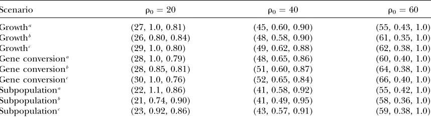
Robustness of approach: To investigate the robust-ness of the likelihood approach using the two-feature sampling distribution, we consider the following three scenarios: (a) population growth, (b) population sub-structure, and (c) gene conversion. For a, we set the starting time point of population expansion to 0.44 (in coalescent units) and the exponential growth rate to
TABLE 1
Estimates ofu
Calling (sn,sp) u0¼200 u0¼400 u0¼600
Dependent (1.0, 1.0) (200, 0.29) (401, 0.23) (596, 0.18) Independent (0.34, 1.0) (200, 0.33) (396, 0.25) (597, 0.23) Dependent (0.34, 1.0) (205, 0.46) (409, 0.31) (608, 0.28) Dependent (0.68, 0.75) (203, 0.59) (408, 0.34) (613, 0.28)
2.1, the maximum-likelihood estimates for this scenario obtained in Plagnolet al. (2006). For b, we choose two settings to test: two equal-sized subpopulations with scaled migration parameter 1.5 (results not shown) and four equal-sized subpopulations with scaled migration parameter 3.0, chosen to achieve average Fst-values of 0.25 (Hudsonet al. 1992). In each case the sample was assumed to be divided equally between the subpopula-tions. For c, we use the estimates in Plagnolet al. (2006) to set the mean length of a conversion tract to 100 bp and the ratio of conversion to crossing-over rates to 4.
Table 3 lists estimates ofr for these three scenarios. We see that we can still estimaterif there is exponential growth, gene conversion, or population structure, pro-vided that we have good estimates of the demographic parameters. Moreover, we can see that we tend to overestimate r when population growth or gene
con-version is present, while there is little bias in the case of population structure.
We emphasize that these scenarios are intended to be exploratory rather than exhaustive. A more extensive test of robustness would examine the effects of changes to mutation, migration and recombination parameters, sample size, and different minor allele frequencies used in obtaining the two-locus sampling distribution.
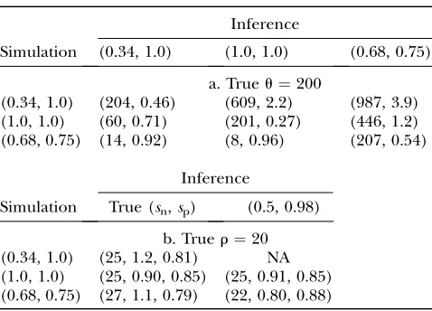
To address the model misspecification question,i.e., what happens if we analyze data under the wrong model or with the wrong sensitivity and/or specificity, we show the effects of using incorrect sensitivity or specificity in Table 4. The main observation is that both our approaches suffer in this case. We show that dependent modeling is more appropriate for SFP experiments (cf. Figure 3) in thediscussion.
We generated test data underu¼200 andr¼20 for a 100-kb region with particular sensitivity and specificity (Table 4, a and b, column 1) and then estimated eitheru orrwith different sensitivity and specificity. For exam-ple, given the true value ofu¼200 we estimateduwith three different combinations of sensitivity and speci-ficity, and we see that only inference using the true parameters (numbers on the diagonal in Table 4a) provides accurate estimates. On the other hand, we also generated the two-feature sampling distribution with parameters similar to the real experimental setting,i.e., sensitivity¼0.50 and specificity¼0.98, and then used this lookup table to estimate r in the test data sets generated with different sensitivity and specificity. For the data sets generated under sn¼0.34 andsp¼1.0, most of the estimates returned are 0, and we label this case ‘‘NA,’’i.e., not applicable. For the other two cases, the estimates seem to be unaffected.
In summary, one needs to obtain reliable estimates of sensitivity and specificity, for example, by sequence comparison, for successful inference.
TABLE 2
Estimates ofr
Type r0¼20 r0¼40 r0¼60
Modifieda (25, 0.90, 0.85) (46, 0.57, 0.91) (63, 0.38, 1.0)
Modifiedb (25, 1.1, 0.81) (43, 0.62, 0.89) (59, 0.41, 1.0)
Modifiedc (27, 1.1, 0.79) (48, 0.62, 0.88) (65, 0.40, 1.0)
Simpleb (27, 1.2, 0.80) (44, 0.60, 0.89) (57, 0.41, 1.0)
Simplec (3, 0.85, 0.99) (16, 0.77, 0.98) (41, 0.56, 1.0)
Realb (22, 1.1, 0.84) (38, 0.62, 0.91) (50, 0.46, 1.0)
Realc (20, 0.95, 0.87) (37, 0.60, 0.94) (52, 0.46, 1.0)
The three numbers within the parentheses denote the mean, the root (relative) mean square error, and probability that the estimate falls within a factor of two of the true param-eter, respectively. Three combinations of (sensitivity, specific-ity) are examined:
a(1.0, 1.0). b
(0.34, 1.0).
c
(0.68, 0.75).
TABLE 3
Robustness of estimates ofr
Scenario r0¼20 r0¼40 r0¼60
Growtha (27, 1.0, 0.81) (45, 0.60, 0.90) (55, 0.43, 1.0)
Growthb (26, 0.80, 0.84) (48, 0.58, 0.90) (61, 0.35, 1.0)
Growthc (29, 1.0, 0.80) (49, 0.62, 0.88) (62, 0.38, 1.0)
Gene conversiona (28, 1.0, 0.79) (48, 0.65, 0.86) (60, 0.40, 1.0)
Gene conversionb (28, 0.85, 0.81) (51, 0.60, 0.87) (64, 0.38, 1.0)
Gene conversionc (30, 1.0, 0.76) (52, 0.65, 0.84) (66, 0.40, 1.0)
Subpopulationa (22, 1.1, 0.86) (41, 0.58, 0.92) (55, 0.42, 1.0)
Subpopulationb (21, 0.74, 0.90) (41, 0.49, 0.95) (58, 0.36, 1.0)
Subpopulationc (23, 0.92, 0.86) (43, 0.57, 0.91) (59, 0.38, 1.0)
Notation is as in Table 2. See text for details. Simulations are run under dependent calling, with probe cov-erage of 3.3% and three combinations of (sensitivity, specificity):
a
(0.34, 1.0).
b
(1.0, 1.0).
c
DISCUSSION
We have shown that single-feature polymorphism data can be used effectively to infer aspects of the population history ofA. thaliana. Single-feature polymorphisms, as a new type of polymorphism data, have certain advantages over other types of polymorphism data. By exploiting the high-throughput nature of arrays, large amounts of polymorphism data can be produced in an economic and efficient way. Given recent advances in the technol-ogy, the probe coverage over the genome of interest can be easily increased (Borevitz and Ecker 2004). New
commercially available tiling arrays cover the reference strain Col with very small spacing (10 bp) between probes. This will help expedite the exploration of natural variation at the genomewide scale.
By taking account of the transformation from SNPs to SFPs, one could apply most of the methods developed for SNP data to SFP data. For example, the product of approximate conditional-likelihood (PACL) approach in Liand Stephens(2003) could be applied by adding one more step reflecting SFP calling after simulating the SNP sample. Moreover, we could use sliding windows across the genome to study variation in mutation rate and recombination rate using SFP data, as well as to find recombination hot spots, provided that there is a rea-sonably dense probe coverage of the region of interest (Fearnheadet al. 2004). Other statistics defined for SNP data, such as Tajima’sDand the inbreeding coefficient, might be derived in an analogous way and used to study natural selection and/or population structure. One appealing and challenging task is to develop methods for using SFPs for fine-mapping purposes. For example, methods such as the spatial clustering scheme in Molitor
et al. (2003), based on haplotype sharing, can be adopted by defining a new metric that takes into account the uncertainty due to SFP calling (Kimet al. 2006).
When considering how best to improve microarray experiment technology and design in our context, we first observe that increasing the specificity leads to larger improvement in accuracy than increasing the sensitivity. This is because the inference is considerably affected by false positive calls. Thus controlling the false discov-ery rate in any statistical approach that calls SFPs is important. To improve modeling of the SFP calling procedure, one could allow for the existence of multiple SNPs within a probe when deriving analytic formulas. In fact, the proportion of probes having more than one SNP in our simulations ranges from 4 to 12% as u increases from 200 to 600, while Nordborget al. (2005) reports that less than one-sixth of the true positive SFPs have more than two alleles. Moreover, the rate at which a probe hybridizes is likely affected by the position of the SNP within the 25-bp region (Borevitzet al. 2003).
It is also important to study the effect of the de-pendent/independent calling schemes. To investigate this, we obtained 406 SFP loci and their corresponding SNPs by comparing SFP calls with the available sequence data for the 16 accessions in our experiment. We then calculated the correlation between the SNP and SFP calls at each SFP locus. Figure 3 gives a histogram showing that the degree of correlation is close to 1, which is very similar to the histogram obtained from simulations under de-pendent calling (histogram not shown). On the other hand, simulations show that for independent calling with parameters matching real experiments, there is sub-stantial mass to both the left and the right of 0 (histogram not shown). Therefore, the mass at 1 tells us that calling is generally quite dependent.
Figure3.—Histogram of correlation coefficients between
SFPs and underlying SNPs for the 406 called features in a real experiment.
TABLE 4
Model misspecification effect in dependent model with 3.3% probe coverage
Inference
Simulation (0.34, 1.0) (1.0, 1.0) (0.68, 0.75)
a. Trueu¼200
(0.34, 1.0) (204, 0.46) (609, 2.2) (987, 3.9) (1.0, 1.0) (60, 0.71) (201, 0.27) (446, 1.2) (0.68, 0.75) (14, 0.92) (8, 0.96) (207, 0.54)
Inference
Simulation True (sn,sp) (0.5, 0.98)
b. Truer¼20 (0.34, 1.0) (25, 1.2, 0.81) NA (1.0, 1.0) (25, 0.90, 0.85) (25, 0.91, 0.85) (0.68, 0.75) (27, 1.1, 0.79) (22, 0.80, 0.88)
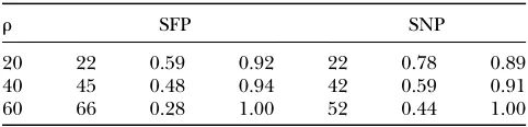
Finally, we have performed a further simulation study to address how much information is lost in inference when using SFP data rather than SNP data. We first simulated coalescent samples of 20 haplotypes, in a 100-kb region. Then SFPs were generated from the SNPs under dependent calling, with coverage 70%, sensitivity 50%, and specificity 95%, as in the current experimental setup. Moreover, we selected candidate SNPs from the SNP sample at a density of 1/10 kb with minor allele frequency .10%. To estimate the recombination pa-rameterr, we applied the two-locus/feature sampling distributions on the selected SNP pairs and called SFP pairs, respectively. The results in Table 5 indicate that SFPs slightly outperform SNPs in this case: the SFPs have a smaller RMSE and a larger proportion of estimates lying within a factor of two of the truerthan those of the SNPs.
We thank two anonymous referees for their helpful comments. This work was funded in part by National Institutes of Health grants HG002790, GM67243, and GM069890. S.T. is a Royal Society–Wolfson Research Merit Award holder.
LITERATURE CITED
Borevitz, J. O., and J. R. Ecker, 2004 Plant genomics: the third
wave. Annu. Rev. Genomics Hum. Genet.55:443–477. Borevitz, J. O., D. Liang, D. Plouffe, H. Chang, T. Zhu et al.,
2003 Large-scale identification of single-feature polymorphisms in complex genomes. Genome Res.13:513–523.
Fearnhead, P., 2003 Consistency of estimators of the
population-scaled recombination rate. Theor. Popul. Biol.64:67–79. Fearnhead, P., R. Harding, J. Schneider, S. Myersand P. Donnelly,
2004 Application of coalescent methods to reveal fine-scale rate variation and recombination hotspots. Genetics167:2067–2081. Griffiths, R. C., and S. Tavare´, 1998 The age of a mutation in a
general coalescent tree. Stoch. Models14:273–295.
Hudson, R. R., 1983 Properties of a neutral allele model with
intra-genic recombination. Theor. Popul. Biol.23:183–201. Hudson, R. R., 2001 Two-locus sampling distributions and their
application. Genetics159:1805–1817.
Hudson, R. R., 2002 Generating samples under a Wright-Fisher
neutral model. Bioinformatics18:337–338.
Hudson, R. R., M. Slatkinand W. Maddison, 1992 Estimation of
lev-els of gene flow from DNA sequence data. Genetics132:583–589. Kim, S., K. Zhao, R. Jiang, J. Molitor, J. O. Borevitz et al.,
2006 Association mapping with single-feature polymorphisms. Genetics173:1125–1134.
Kingman, J. F. C., 1982 The coalescent. Stoch. Proc. Appl.13:235–248.
Li, N., and M. Stephens, 2003 Modeling linkage disequilibrium and
identifying recombination hotspots using single-nucleotide poly-morphism data. Genetics165:2213–2233.
McVean, G. A., S. R. Myers, S. Hunt, P. Deloukas, D. R. Bentley
et al., 2004 The fine-scale structure of recombination rate vari-ation in the human genome. Science304:581–584.
Molitor, J., P. Marjoramand D. Thomas, 2003 Application of
Bayes-ian clustering via Voronoi tesselations to the analysis of haplotype risk and gene mapping. Am. J. Hum. Genet.73:1368–1384. Nordborg, M., 2001 Coalescent theory, pp. 179–208 inHandbook
of Statistical Genetics, edited by D. J. Balding, M. J. Bishopand
C. Cannings. John Wiley & Sons, New York.
Nordborg, M., T. T. Hu, Y. Ishino, J. Jhaveri, C. Tanget al.,
2005 The pattern of polymorphism in Arabidopsis thaliana. PLoS Biol.3:e196.
Parmigiani, G., E. S. Garett, R. A. Irizarryand S. L. Zeger
(Edi-tors), 2003 The Analysis of Gene Expression Data: Methods and Soft-ware. Springer-Verlag, New York.
Plagnol, V., B. Padhukasahasram, J. D. Wall, P. Marjoramand
M. Nordborg, 2006 Relative influences of crossing over and
gene conversion on the pattern of linkage disequilibrium in
Arabidopsis thaliana. Genetics172:2441–2448.
Speed, T. P. (Editor), 2003 Statistical Analysis of Gene Expression
Micro-array Data. Chapman & Hall/CRC Press, London/New York/ Cleveland/Boca Raton, FL.
Storey, J. D., and R. Tibshirani, 2003 Statistical significance for
ge-nomewide studies. Proc. Natl. Acad. Sci. USA100:9440–9445. Tajima, F., 1983 Evolutionary relationship of DNA sequences in
fi-nite populations. Genetics105:437–460.
Tusher, V. G., R. Tibshiraniand G. Chu, 2001 Significance analysis
of microarrays applied to the ionizing radiation response. Proc. Natl. Acad. Sci. USA98:5116–5121.
Wall, J. D., 2000 A comparison of estimators of the population
re-combination rate. Mol. Biol. Evol.17:156–163.
Watterson, G. A., 1975 On the number of segregating sites in
genetical models without recombination. Theor. Popul. Biol.7:
256–276.
Weiss, G., and A.vonHaeseler, 1998 Inference of population
his-tory using a likelihood approach. Genetics149:1539–1546. Werner, J. D., J. O. Borevitz, N. Warthmann, G. T. Trainer, J. R.
Eckeret al., 2005 Quantitative trait locus mapping and DNA
array hybridization identify an FLM deletion as a cause for natu-ral flowering-time variation. Proc. Natl. Acad. Sci. USA 102:
2460–2465.
Wolyn, D., J. O. Borevitz, O. Loudet, C. Schwartz, J. Maloof
et al., 2004 Light-response quantitative trait loci identified with composite interval and eXtreme array mapping in Arabidopsis thaliana. Genetics167:907–917.
Communicating editor: G. Gibson
TABLE 5
Estimates of the population recombination raterin a 100 kb region
r SFP SNP
20 22 0.59 0.92 22 0.78 0.89
40 45 0.48 0.94 42 0.59 0.91
60 66 0.28 1.00 52 0.44 1.00
The SNP case has density one every 10 kb and the SFP case has 70% coverage, 95% specificity, and 50% sensitivity under a dependent calling scheme. In each of the SFP and SNP cate-gories, first column gives the average estimate, the second the RMSE, and the third the proportion of estimates lying within a factor of 2 of the truth.
APPENDIX
An illustration of the SFP-calling procedure: Under independent calling, true/false positive/negative calls are independent between accessions at a given probe position, while there are only four possibilities under dependent calling,i.e.,
I. 1/1 and 0/0; II. 1/0 and 0/1; III. 1/1 and 0/1; IV. 1/0 and 0/0.
Here we illustrate a case in which SFP calling is assumed to be dependent across accessions. Suppose we have four accessions plus the reference and are in-terested in a region of three distinct probes. We simulate a sample of five haplotypes, noting again thatA. thaliana
variation for each accession. The haplotypes are repre-sented by the five rows in Figure A1, where 0 denotes wild type and 1 denotes mutant. The top row is chosen randomly as the reference, and the other four are accessions. Assuming that there is exactly one SNP within each probe, this results in the haplotypes shown in the left part of Figure A1, labeled ‘‘SNP.’’ We then undertake the SFP comparison phase by comparing the accessions with the reference (the top row). In this phase we use 1 to indicate a location that is different from the reference probe and 0 otherwise. By doing so we get the middle matrix, labeled ‘‘*.’’ Note that only the first column has been changed since the chosen reference contained the derived mutation in this case. Finally, we apply the SFP-calling phase to the middle matrix to obtain the SFP matrix on the right, where 1 denotes a called significant difference between the accession probe and the reference probe and 0 anything else. This illustrates a calling operation of type III at the first probe position, type I at the second probe position, and type II at the last probe position. Calling operations of type I represent true calls, so every comparison remains the same. Calling operations of type II in-troduce false negatives and false positives, which flip 0’s to 1’s and vice versa. Type III introduces only false positives, which flip 0’s to 1’s. When the sensitivity and specificity are both 1.0,i.e., the ideal case, the middle matrix is the same as the SFP matrix.
The expected number of SFPs: Denote the probe configuration byP ¼ ðP1;P2;. . .;PnpÞ, wherenpis the
number of probes, andPi¼1 if theith probe is called an
SFP or 0 otherwise. Recall that an SFP is called at theith probe if and only if at least one accession is called polymorphic with respect to the reference. Denote the total number of SFPs called by F. Then we have
F ¼Pnp
i¼1Piand
E½F ¼E X
np
i¼1
Pi " #
¼X np
i¼1
E½Pi ¼X
np
i¼1
PðPi¼1Þ; ðA1Þ
where E[] stands for mathematical expectation and P() stands for probability.
Conditional on the number of SNPs within a partic-ular probe, the probe setPcan be partitioned into two parts, probes containing one SNP and probes without SNPs, denoted by P1 and P0, respectively. That is, P ¼ P1[ P0. Following Equation A1, we have
E½F ¼X
i2P1
PðPi¼1Þ1 X
j2P0
PðPj¼1Þ
¼ajP1j1bjP0j; ðA2Þ
wherejAjdenotes the size of the setA,a¼PðPi ¼1j P1Þ,
andb¼PðPi ¼1j P0Þ. Recall that we assume that probes
are called independently.
Next, we compute the probabilities a and b. First, consider a probe with one and only one segregating site inside. The mutation within the probe partitions the sample into two groups, the wild-type group and the mutant group. For example, there are three wild types and two mutants in the first probe in Figure A1 (the first column in the SNP matrix). Letqnbdenote the
proba-bility of obtainingbmutants out ofnindividuals, which is given in Griffithsand Tavare´(1998). Recall that an SFP is called if and only if at least one 1 appears in the resulting SFP matrix (the right part in Figure A1). In other words, the only way of not calling an SFP is to have true negative calls and false negative calls at the probe position, by applying calling operation IV (1/0 and 0/0) on each accession probe (cf. the middle section in Figure A1). Conditioning on which group the reference is chosen from, we have
a¼
Pn1
b¼1qnb½ð1 ð1snÞnbspb1Þnb
1ð1 ð1snÞbspnb1Þn
b
n ; independent calling;
1 ð1snÞsp; dependent calling:
8 > < > :
ðA3Þ
For a probe containing no SNP, the chance of being called an SFP is determined by the specificity. There-fore, we have
b¼ 1sn
1
p ; independent calling; 1sp; dependent calling:
ðA4Þ
Finally, assuming that there is at most one SNP within a probe, we can determine the size of the set of probes with SNPs; i.e., jP1j ¼S, where S is the number of segregating sites or SNPs. Following Equation A2, we obtain
E½F jS ¼ajP1j1bjP0j ¼aS1bðnpSÞ; ðA5Þ
wherenpis the total number of probes. Furthermore, we have
E½F ¼E½E½FjS ¼npb1ðabÞE½S
¼npb1ðabÞ
npLp
L
Xn1
k¼1 1
ku; ðA6Þ
Figure A1.—Example of transforming SNP data to SFP
where the last term is given under the infinite-sites mutation model (Watterson 1975), and Lp is the length of a probe (i.e., 25 bp) andLis the total length of the region in base pairs.
Obtaining two-feature SFPs from SNPs: Figure A2 illustrates how different SNP configurations can lead to the same SFP configuration. Suppose that we have a sample of 19 accessions plus the reference, i.e., the sample size is 20. Suppose further that calling is completely dependent across accessions. We focus on a particular pair of features, where we assume there is one and only one segregating site within each feature. First we explain the top part in Figure A2, where there are 3 00’s, 5 01’s, 7 10’s, and 5 11’s at the two segregating sites in the sample. Assume that the type of the ref-erence is randomly chosen to be 00. Then after the SFP comparison phase, all the combinations remain the same in the * matrix. Furthermore, if both calling op-erations at the two features are of type I, i.e., true positive/negative only, we again obtain the SFP config-urationm¼(3, 5, 7, 5). For the case where the reference is not of type 00, we look at the middle section in Figure A2. Suppose that we have a different SNP configuration, n¼(5, 3, 5, 7), and the type of the reference is 01. Thus in the SFP comparison phase, the original combination 00 becomes 01 compared to the reference 01, and 01 becomes 00, etc. As can be seen, the * matrix will lead to the same SFP configuration,m¼(3, 5, 7, 5), if we have
both calling operations of type I. Similarly, we can see in the bottom part of Figure A2, where the reference is again 00 but now the second feature uses a calling operation of type II, how a different SNP configuration can give rise to such an SFP configuration by taking appropriate calling operations at the two features.
Although there are four possible calling operations altogether, only the first three lead to an SFP in the resulting sample, since, assuming completely depen-dent calling, operation IV changes the column of that probe to all 0’s. For given sensitivity and specificity, we can write down the probability for each calling opera-tion,e.g.,P(CI)¼snsp.
We noted earlier that under the completely depen-dent calling assumption, the false positives have one common pattern in the resulting SFP matrix,i.e., all 1’s but one 0 for the reference probe. To see this, start from a probe without any SNP in it. After the SFP comparison phase, the probes at this position are all labeled by 0, since there is no polymorphism among them. In the SFP calling phase, if one of the accession probes is called significantly different,i.e., 0/1, then the rest of the accession probes are also called significantly dif-ferent, under dependent calling. Thus this probe is called as an SFP, however, a false positive. On the other hand, the only SNP configuration that could give rise to the above pattern is (0, 1, 1,. . ., 1) (without loss of generality, we label the first one as wild type and the rest as mutants). In this case the reference is most likely to be chosen from the mutant group, in which case this column becomes (1, 0, 0,. . ., 0) after the SFP compar-ison phase. Furthermore, the only operation that can change this column to the pattern of false positives is of type III,i.e., (1/1 and 0/1). This is the only situa-tion that a probe with segregating sites can lead to the same pattern as a false positive. However, the probability of obtaining only one wild type in the infinite-sites model is very small, in particular when the sample size is large.
Consistency of MLE of r: The consistency of the maximum-likelihood estimates ofrcannot be shown for the general setting in the two-feature sampling distri-bution. However, it can be shown that if we modify the approach by insisting that all pairs of features be within a certain distance we would obtain consistent estimates of r, as in the modified approach of the two-locus sampling distribution. The key point of the additional restriction is that linkage disequilibrium decays inversely to the distance between two sites. The proof in Fearnhead (2003) can be adopted without substantial change. The adjustment is in Lemma 5, in which we need to sum over all possible two-loci SNP configurations to compute the covariance coefficients between two features. Recall that there are only four possibilities in the modified two-feature sampling derivation and nine possibilities in the simple two-feature sampling derivation. Thus, the con-clusion holds in the SFP setting.
FigureA2.—Example of different two-locus configurations
Statistical properties of the two-feature sampling dis-tribution:One way to study the statistical properties of the maximum-likelihood estimate ˆr is to consider the minimal contrast,i.e., the expectation of logr0ðpcðm;rÞÞ, over the distribution ofmconditional on polymorphism at both features (cf. Hudson2001). That is, we consider
Er
0½logðpcðm;rÞÞ ¼ X
m
pcðm;r0Þlogðpcðm;rÞÞ: ðA7Þ
The plots of the above function (not shown here) show that the likelihood curve has a peak at a position close to the true value r0, which enables the maximum-likeli-hood approach to work.
To study the asymptotic variance of the maximum-likelihood estimate of r0, we compute the second derivative of the function in (A7) with respect to r, evaluated at the r0, assuming k pairs of features are considered. That is, we compute
Varr0;kðˆrÞ
1 kð@2=@r2ÞEr
0ðlogpcðm;rÞÞ jr¼r0
: ðA8Þ
An approximation of the above is plotted in Figure A3. The curves of estimated variance in both the SNP case and the SFP case are similar; however, there is smaller variance in the SNP case than in the SFP case, since there is more randomness in the latter. The asymptotic plot shows that features separated byrin the range of 2– 15 are best for estimating r, as is observed also in Hudson(2001).
Note that the difference between the scales in Figure A3 and the corresponding figure in Hudson(2001) is due to different conditionings on the two sites when
obtaining the two-locus sampling distribution. Hudson (2001) restricted to those sites where the minor allele frequency is.10%, where we require just that both sites are segregating. In other words, the minor allele frequency is .5% (i.e., 1 of 20) in our scheme. Since the ages of SNPs are related to their frequencies, SNPs with larger frequency tend to be older than those with smaller frequency, so they are more informative about recombination than rarer SNPs. As a result, condition-ing on the minor allele frequency.10% leads to smaller variance of MLEs than those conditional on minor allele frequency.5%.
FigureA3.—Estimates of the asymptotic variance of log ˆr