DOI: 10.1534/genetics.107.085753
A Two-Stage Pruning Algorithm for Likelihood Computation for a
Population Tree
Arindam RoyChoudhury,*
,1Joseph Felsenstein
†and Elizabeth A. Thompson
‡*Department of Organismic and Evolutionary Biology, Harvard University, Cambridge, Massachusetts 02138 and†Department of Genome Sciences and‡Department of Statistics, University of Washington, Seattle, Washington 98195
Manuscript received December 11, 2007 Accepted for publication August 8, 2008
ABSTRACT
We have developed a pruning algorithm for likelihood estimation of a tree of populations. This algorithm enables us to compute the likelihood for large trees. Thus, it gives an efficient way of obtaining the maximum-likelihood estimate (MLE) for a given tree topology. Our method utilizes the differences accumulated by random genetic drift in allele count data from single-nucleotide polymorphisms (SNPs), ignoring the effect of mutation after divergence from the common ancestral population. The computation of the maximum-likelihood tree involves both maximizing likelihood over branch lengths of a given topology and comparing the maximum-likelihood across topologies. Here our focus is the maximization of likelihood over branch lengths of a given topology. The pruning algorithm computes arrays of probabilities at the root of the tree from the data at the tips of the tree; at the root, the arrays determine the likelihood. The arrays consist of probabilities related to the number of coalescences and allele counts for the partially coalesced lineages. Computing these probabilities requires an unusual two-stage algorithm. Our computation is exact and avoids time-consuming Monte Carlo methods. We can also correct for ascertainment bias.
A
LLELE-COUNT data, the number of occurrences of each allele, are often used by researchers to estimate the evolutionary tree. Likelihood estimation of the evolutionary tree from allele-count data was introduced by Edwards and Cavalli-Sforza (1964)and Cavalli-Sforza and Edwards (1967), followed
by D. Gomberg (unpublished results). They used a
Brownian-motion approximation for genetic drift. Felsenstein(1968, 1973a,b) introduced the
‘‘prun-ing’’ algorithm, for the Brownian-motion approximation leading to an efficient calculation. Thompson (1975)
also used a form of pruning algorithm for likelihood estimation of branch lengths of an evolutionary tree. The idea of pruning (or ‘‘peeling,’’ as it is commonly known in studies of pedigrees in statistical genetics) also appears in the work of Hilden(1970). Elstonand Stewart(1971)
introduced peeling upward in a pedigree. Heuchand Li
(1972) introduced peeling upward and downward alter-nately for an unlooped pedigree.
Nielsen et al. (1998) and Nielsen and Slatkin
(2000) introduced an exact likelihood-based method of estimating the evolutionary tree using the coalescent. They devised a method of computing the likelihood of trees with specified structures (called topologies) and specified branch lengths. The branch lengths are time
in generations, scaled by effective population size. They computed the likelihood for a given combination of numbers of coalescent events in each branch and then summed over all possible combinations of these num-bers. They ignored the effect of mutation after di-vergence from the common ancestral population. They maximized the likelihood first over the branch lengths within each topology and then over the topol-ogies. However, their summations over the number of coalescent events of the branches have a complicated nested pattern that makes it algebraically intractable for a tree with five or more populations. The coalescent model they used to model the process of evolution is not reversible. Irreversibility of their model makes it possi-ble to model the direction of time in the tree. As a result they are able to estimate a rooted tree. In other words, they were able to estimate the earliest point in the tree, in addition to the tree.
In this article we put the model of Nielsen et al.
(1998) in a form that takes into account the conditional-independence structure of the coalescent tree. By doing so we are able to devise a pruning algorithm for the tree of populations. Pruning leads to an efficient algorithm for dealing with the nested summations described in the previous paragraph. Thus, we are able to compute the likelihood of a tree with a large (five or more) number of populations. A similar approach has been developed by David Bryant and Noah Rosenberg (D. Bryantand
N. Rosenberg, personal communication).
1Corresponding author:Wakeley Lab, 4092-4100 Biological Laboratories,
16 Divinity Ave., Harvard University, Cambridge, MA 02138. E-mail: [email protected]
Our theory is applicable to both diploid and haploid organisms although our sampling unit is haploid, a set of chromosomes formed by one chromosome of each kind. For a haploid organism chromosomes from each individual form one haploid sampling unit, while for a diploid organism chromosomes from each individual form two haploid sampling units.
We developed our method to analyze allele count at a set of single-nucleotide polymorphism (SNP) loci, where the allele count for each locus is statistically independent of that for any other locus. Henceforth we use the term ‘‘independent loci’’ to refer to such a set of loci. As in Nielsenet al.(1998), our branch lengths are
time in generations, scaled by effective population size. The definition of branch length comes from the fact that the rate of coalescence depends on the time scaled by effective population size. Note that if we assume a Moran model for the population, then the time scaled by population size would bet=2N; for a Wright–Fisher model it will bet=N (Moran1962). Heretis time andN
is the (haploid) population size. This difference arises due to the fact that a Moran model has twice as much genetic drift (for the same period of time) as a Wright– Fisher model with the same population size. Since we are using the evolutionary model of Nielsen et al.
(1998), we also estimate a rooted tree.
We can also correct for ascertainment. Correcting for ascertainment is important, as data only from ascer-tained SNPs are available in practice. Although it is not the focus of this article, we briefly outline the ascertain-ment correction process in the implementing an ascertainment correctionsection.
A PRUNING ALGORITHM
In this section we address the computation of the likelihood for given branch lengths in a given topology. Suppose that we have allele-count data forL indepen-dent SNP loci, each with two alleles, ‘‘0’’ and ‘‘1.’’ Note that we do not assume that we know which of the two alleles is ancestral; we assign the labels 0 and 1 arbitrarily. The likelihood based on all loci would be the product of likelihoods computed from each of theL loci, one at a time. It thus suffices to devise a method of computing the likelihood for one locus.
Suppose we have allele-count data from P different populations. For a given locus, let s¼ ðs1;s2;. . .;sPÞ
denote the vector of allele counts. The quantitysiis the
allele count (the count of 1 alleles) in a sample ofmi
haploid genotypes from theith population. The likeli-hood based on this particular locus would be
LðtÞ ¼Prðs¼ ðs1;s2;. . .;sPÞ jtÞ:
Here t¼ ðt1;t2;. . .;tð2P2ÞÞ is the vector of branch
lengths. As we go back in time along the branches toward the root, the lineages coalesce with each other.
The straightforward method (Nielsen et al. 1998;
Nielsen and Slatkin 2000) of computing the
likeli-hood involves conditioning on the (random) numbers of coalescent events at each branch,
PrðsjtÞ
¼X
k1 X
k2
. . . X kð2P2Þ
PrðsjK1¼k1;K2¼k2;. . .;Kð2P2Þ¼kð2P2ÞÞ
3PrðK1¼k1;K2¼k2;. . .;Kð2P2Þ¼kð2P2ÞjtÞ; ð1Þ
whereKxis the number of coalescent events in branchx,
and the sum is over allk1;k2;. . .;kð2P2Þ such that they
represent a set of possible values forK1;K2;. . .;Kð2P2Þ
givenðm1;m2;. . .;mPÞ. (The exact set of possible values
depends on the topology.) Note that there are only finitely many possibilities forðk1;k2;. . .;kð2P2ÞÞ;
there-fore it is theoretically possible to compute the summa-tion at the right-hand side of Equasumma-tion 1 exactly. However, the large number of terms in the summation makes the likelihood hard to evaluate for a large tree. Here we present a pruning algorithm as an efficient way of computing this likelihood.
To use this algorithm, we need to keep track of two sets of probabilities for each node in the tree. The first consists of the probabilities of numbers of lineages ancestral to our samples at each internal node in the tree. The second set consists of the probabilities of the samples descended from each node in the tree, condi-tional on different numbers of lineages ancestral to each allele at that node. The calculations of these two different sets of probabilities flow in opposite direc-tions. In the first set there are the probabilities of some unobserved quantities from the past, conditional on the total number of observations at the present. In the second set there are the probabilities of the observa-tions, conditional on the value of those unobserved quantities from the past. These opposite flows of proba-bilities require the use of a two-stage algorithm. Starting from the most recent branches, we compute the two stages one branch at a time. In the first stage we compute the first set of probabilities for a particular branch. In the second stage Bayes’ theorem is used to reverse the direction of the flow of the first set of prob-abilities and the second set of probprob-abilities is computed thereby for the branch.
Underlying structure: We discuss the pruning
algo-rithm by reference to Figure 1. In Figure 1, the lower a location is in the tree, the more recent it is.
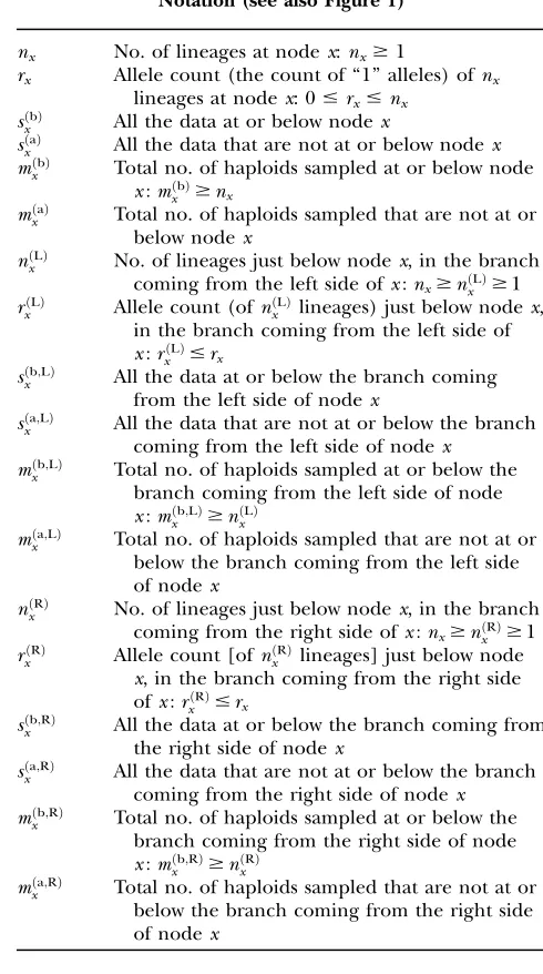
At this point, we introduce our notation for the different random variables used for this article (Table 1 and Figure 1). The random variables of primary interest arenx, the number of lineages at nodex, and
rx, the allele count (of nx lineages) at node x. We
considered also mðbÞ
x , the total number of haploid
individuals sampled at or below node x, and sðbÞ
x , all
data observed at or below a particular time point in the tree, conditioned on the allelic configuration at that time point. Next we use the term ‘‘a location just below a node, in the branch coming from the left (or the right) side of node x,’’ to mean a time-point x9 at the left branch (or the right branch), such that the time period betweenxandx9is infinitesimally small (and, therefore, no coalescent event has taken place in that period).
Our pruning algorithm computes arrays of probabil-ities at each node of a tree. First, the arrays of the probabilities are computed at each tip from the data at that tip. Then the arrays of probabilities at a location (a node or a location just below a node) are computed on the basis of the location(s) just below that one (see Figure 1). By repeating this process, we eventually reach the root of the tree, where the likelihood is computed from the arrays of probabilities at the root.
At a location (at a nodex, or just below a nodex, in one of the two branches) there are two arrays of probabilities related to the number of coalescence events and the allele counts among the partially co-alesced lineages. The first array consists of the proba-bilities of different numbers of lineages at that location. The probabilities are computed from the lengths of the branches between that location and the present. The second array consists of the conditional probability of the data observed at or below that location, conditional on the possible numbers of lineages in that location and the possible allele counts at those lineages. To be specific, the first array at a nodexis given by
AðxÞ ¼ ðPrðnx¼iÞ;i¼1;2;. . .;mxðbÞÞ;
so that
AðxÞi¼Prðnx¼iÞ:
The second array at a nodexis two dimensional and is given by
BðxÞ ¼ ððPrðsðbÞ
x jnx ¼i;rx¼jÞ;j ¼0;1;2;. . .;iÞ;
i¼1;2;. . .;mðxbÞÞ;
so that
BðxÞij¼PrðsðbÞ
x jnx ¼i;rx¼jÞ:
Note that the probabilities in the components of A(x) andB(x) are computed conditional on the topology, the branch lengths, and the sample sizes in the tips below node x. However, for notational simplicity we do not explicitly write them as functions of these. At a point just below and coming from the left side of nodex, the first array is given by
AðLÞðxÞ ¼ ðPrðnðLÞ
x ¼iÞ;i¼1;2;. . .;m
ðb;LÞ
x Þ;
so that
Figure1.—Structure of an evolutionary tree.
TABLE 1
Notation (see also Figure 1)
nx No. of lineages at nodex:nx$1
rx Allele count (the count of ‘‘1’’ alleles) ofnx lineages at nodex: 0#rx#nx
sðbÞ
x All the data at or below nodex sðaÞ
x All the data that are not at or below nodex mðbÞ
x Total no. of haploids sampled at or below node x:mðbÞ
x $nx mðaÞ
x Total no. of haploids sampled that are not at or below nodex
nðLÞ
x No. of lineages just below nodex, in the branch coming from the left side ofx:nx$nxðLÞ$1 rðLÞ
x Allele count (ofn
ðLÞ
x lineages) just below nodex, in the branch coming from the left side of x:rðLÞ
x #rx sðb;LÞ
x All the data at or below the branch coming from the left side of nodex
sða;LÞ
x All the data that are not at or below the branch coming from the left side of nodex
mðb;LÞ
x Total no. of haploids sampled at or below the branch coming from the left side of node x:mðb;LÞ
x $n
ðLÞ
x mða;LÞ
x Total no. of haploids sampled that are not at or below the branch coming from the left side of nodex
nðRÞ
x No. of lineages just below nodex, in the branch coming from the right side ofx:nx$nxðRÞ$1 rðRÞ
x Allele count [ofn
ðRÞ
x lineages] just below node x, in the branch coming from the right side ofx:rðRÞ
x #rx sðb;RÞ
x All the data at or below the branch coming from the right side of nodex
sða;RÞ
x All the data that are not at or below the branch coming from the right side of nodex mðb;RÞ
x Total no. of haploids sampled at or below the branch coming from the right side of node x:mðb;RÞ
x $n
ðRÞ
x mða;RÞ
AðLÞðxÞi ¼PrðnðLÞ
x ¼iÞ;
and the second array is given by
BðLÞðxÞ ¼ ððPrðsðb;LÞ
x jn
ðLÞ
x ¼i;r
ðLÞ
x ¼jÞ;j¼0;1;2;. . .;iÞ;
i¼1;2;. . .;mxðb;LÞÞ;
so that
BðLÞðxÞij ¼Prðsðb;LÞ
x jn
ðLÞ
x ¼i;r
ðLÞ
x ¼jÞ:
A(R)(x) andB(R)(x) are similarly defined for a point just
below and coming from the right side of nodex. Note that the probabilities in the components of A(L)(x),
B(L)(x), A(R)(x), and B(R)(x) are computed conditional
on the topology, the branch lengths, and the sample sizes in the tips below nodex. As in the cases ofA(x) and B(x), for notational simplicity we do not explicitly write them as functions of these.
At a tipxthe arrays of probabilities can be obtained using the fact that
Prðnx¼iÞ ¼1ði¼mxÞ
and that
PrðsðbÞ
x jnx¼i;rx ¼jÞ ¼1ði¼mx;j¼sxÞ;
wheresx is the allele count observed at the tipx, in a
sample ofmxhaploids. Starting from the tips, the arrays
of probabilities from the tips upward are computed recursively using two different steps. These steps are shown in Figure 2. Step 1 computes the arrays of probabilities at a location just below the top of a branch from those at the bottom node of the branch. Step 2 combines the two sets of arrays from just below a node (from the right and from the left), to obtain the arrays of probabilities at that node. The arrays at the root are computed by a final use of step 2. Then we compute the likelihood from the arrays at the root at all loci. In many standard pruning algorithms probabilities of the obser-vations seen at or below a point on the tree are computed conditional on each of the different possible true states at that point (see, for example, Elstonand
Stewart 1971). These are then updated, moving
rootward. Here, the presence of the coalescent, a stochastic process that moves backward in time, leads to an unusual bidirectional conditioning.
Step 1:Consider a branch with bottom nodeyand top
nodez. Step 1 computes the arrays of probabilities at the location in that branch just below z from those at y. Without loss of generality, let us assume that this branch comes tozfrom the left side. Thus, it suffices to have a method for computing A(L)(z) and B(L)(z) from A(y),
B(y) and from the branch length. We use equations involving two different quantities to compute the arrays of probabilities in an upward location of the tree from the arrays of probabilities at some given location(s) of
the tree. One is PrðnðLÞ
z ¼i9jny ¼iÞ, computed from
the branch length tjk. This is given by Takahataand
Nei(1985) as
PrðnðLÞ
z ¼i9jny¼iÞ
¼ Y
i
j¼i911
lj
0 @
1 AXi
j¼i9
eljtyz
Qi
j9¼i9;j96¼jðlj9ljÞ
¼Qii9; ð2Þ
wherelj¼jðj1Þ=2. The second equation is for
Prðry¼jjrzðLÞ¼j9;n
ðLÞ
z ¼i9;ny¼iÞ;
given by Nielsenet al.(1998) as
Prðry¼jjrzðLÞ¼j9;n
ðLÞ
z ¼i9;ny¼iÞ
¼ bðj;ijÞ
bðj9;i9j9Þ ii9
jj9
; ð3Þ
whereb(., .) is the beta function, defined as
bðu;wÞ ¼
ð1 0
tðu1Þð1tÞðw1Þ dt;
which equalsðu1Þ!ðw1Þ!=ðu1w1Þ!if bothuand w are positive integers. Interestingly, these two equa-tions have probability flowing in opposite direcequa-tions. This makes it difficult to obtain a straightforward transition probability. So we split the transition into two stages. At the first stage we compute A(L)(z). The
components ofA(L)(z) are computed as
AðLÞðzÞi9¼Prðn ðLÞ
z ¼i9Þ
¼X
mðybÞ
i¼i9
PrðnðLÞ
z ¼i9jny¼iÞPrðny¼iÞ
¼X
mðybÞ
i¼i9
Qii9AðyÞi; ð4Þ
using Equation 2 above. Then at the second stage we computeB(L)(z). Bayes’ theorem is used to reverse the
direction of conditioning and compute the
ties Prðny¼ijnzðLÞ¼i9Þ, and then these quantities are
used to compute the components ofB(L)(z):
Prðny¼ijnzðLÞ¼i9Þ ¼
PrðnðLÞ
z ¼i9jny¼iÞPrðny¼iÞ
PrðnðLÞ
z ¼i9Þ
¼Qii9AðyÞi
AðLÞðzÞi9: (Note thatnðLÞ
z is independent of the sample sizes, given
ny. Thus,Qii9is free from the sample sizes at the tips.) We
then obtain the components ofB(L)(z) as
BðLÞðzÞij¼Prðsðb;LÞ
z jn
ðLÞ
z ¼i;r
ðLÞ
z ¼jÞ
¼X
mðybÞ
i9¼i
Xi9
j9¼0 PrðsðbÞ
y jny¼i9;ry¼j9Þ
3Prðry¼j9jrzðLÞ¼j;n
ðLÞ
z ¼i;ny¼i9Þ
3Prðny¼i9jnzðLÞ¼iÞ
¼X
mðybÞ
i9¼i
Xi9
j9¼0
BðyÞi9j9Prðry¼j9jrzðLÞ¼j;n
ðLÞ
z ¼i;ny¼i9Þ
3Prðny¼ijnzðLÞ¼i9Þ: ð5Þ
Step 2:Step 2 is analogous to step 1. Step 2 combines
the two sets of arrays {A(L)(x), B(L)(x)} and {A(R)(x),
B(R)(x)} just below node x, to obtain the arrays {A(x),
B(x)} at nodex. We make use of equations to compute two different quantities to make the transition at step 2. One is for Prðnx ¼ijnðxLÞ¼i9;n
ðRÞ
x ¼i$Þ. This is an
indicator function for whether (nðLÞ
x 1n
ðRÞ
x Þ ¼nx. The
other is for PrðrðLÞ
x ¼j9;r
ðRÞ
x ¼j$jrx ¼j;nxðLÞ¼i9;n
ðRÞ
x ¼
i$Þ, which is simply the hypergeometric probability
PrðrðLÞ
x ¼j9;rxðRÞ¼j$jrx¼j;nxðLÞ¼i9;nðxRÞ¼i$Þ ¼ j j9
ij i9j9
i i9
ð6Þ (withi¼i9 1i$andj¼j9 1j$). As in step 1, these two
equations have the conditioning of the probability flowing in opposite directions. Again we split the computation into two stages. At the first stage A(x) is computed. We computeA(x) as
AðxÞi ¼Prðnx ¼iÞ
¼X
i
i9¼0 PrðnðLÞ
x ¼i9ÞPrðn
ðRÞ
x ¼ii9Þ
¼X
i
i9¼0
AðLÞðxÞi9A ðRÞðxÞ
ðii9Þ:
Then at the second stage B(x) is computed. Bayes’ theorem is used to reverse the direction of conditioning and compute the probabilities PrðnðLÞ
x ¼i9;n
ðRÞ
x ¼
i$jnx¼iÞ, and then these quantities are used to
compute the components ofB(x):
PrðnðLÞ
x ¼i9;n
ðRÞ
x ¼i$jnx¼iÞ
¼Prðnx ¼ijnðxLÞ¼i9;n
ðRÞ
x ¼i$Þ
3PrðnðLÞ
x ¼i9ÞPrðn
ðRÞ
x ¼i$Þ=Prðnx¼iÞ
¼1ði¼i91i$ÞA ðLÞðxÞ
i9AðRÞðxÞi$AðxÞ 1
i :
We can then get the components ofB(x) as
BðxÞij¼PrðsðbÞ
x jnx¼i;rx¼jÞ
¼ X
mðxb;LÞ
i9¼1
X
mðxb;RÞ
i$¼1
Xi9
j9¼0
Xi$
j$¼0
Prðsðb;LÞ
x jn
ðLÞ
x ¼i9;r
ðLÞ
x ¼j9Þ
3Prðsðb;RÞ
x jn
ðRÞ
x ¼i$;r
ðRÞ
x ¼j$Þ
3PrðrðLÞ
x ¼j9;r
ðRÞ
x ¼j$jrx¼j;nxðLÞ¼i9;n
ðRÞ
x ¼i$Þ
3PrðnðLÞ
x ¼i9;n
ðRÞ
x ¼i$jnx ¼iÞ
¼ X
mðxb;LÞ
i9¼1
Xi9
j9¼0
Xii9
j$¼0
BðLÞðxÞi9j9B ðRÞðxÞ
ðii9Þj$
3PrðrðLÞ
x ¼j9;r
ðRÞ
x ¼j$jrx ¼j;nðxLÞ¼i9;
nðxRÞ¼ii9Þ:
ð7Þ
These equations are analogous to the corresponding Equation 5 in step 1, but are more complicated as the arrays of probabilities from the two branches are being combined. Equation 7 uses the fact that sðbÞ
x ¼ ðs
ðb;LÞ
x ;
sðb;RÞ
x ) and thats
ðb;LÞ
x ands
ðb;RÞ
x are independent of each
other givennðLÞ
x ,n
ðRÞ
x ,r
ðLÞ
x , andr
ðRÞ
x .
Likelihood from the arrays at the root: For
conve-nience, let us denote the root as node 0. At the root we have arrays given by
Að0Þ ¼ ðPrðn0 ¼iÞ;i¼1;2;. . .;m0Þ
Bð0Þ ¼ ððPrðs0ðbÞjn0¼i;r0¼jÞ;j¼0;1;2;. . .;iÞ;
i¼1;2;. . .;m0Þ:
Using these we can compute the joint likelihood of t and the ancestral allele frequencypas
Lðt;pÞ ¼X
m0
i¼1
Xi
j¼0
PrðData[sð0bÞjn0¼i;r0¼jÞ
3Prðr0¼jjn0¼i;pÞPrðn0 ¼iÞ
¼X
m0
i¼1
Xi
j¼0
Bð0ÞijPrðr0 ¼jjn0¼i;pÞAð0Þi:
Here Pr(r0¼jjn0¼i,p) is the binomial probability,
Prðr0¼jjn0 ¼i;pÞ ¼ i j p
jð1pÞðijÞ:
fbetaðx;z1;z2Þ ¼ 1
bðz1;z2Þx
z11ð1xÞz21:
The quantityuis 4Nem, where the quantities Neandm are the effective population size and the mutation rate, respectively, for the common ancestral population of the populations under consideration. This gives us the marginal likelihood oftas
LðtÞ ¼
ð1 0
Lðt;pÞpðpÞdp
¼X
m0
i¼1
Xi
j¼0
Bð0ÞijAð0Þi i j
ð1 0
pjð1pÞðijÞ
fbetaðp;u;uÞdp
¼X
m0
i¼1
Xi
j¼0
Bð0ÞijAð0Þi i j
bðj1u;ij1uÞ
bðu;uÞ
:
The choice of this beta distribution comes from the fact that the stationary distribution of allele frequency over loci has this distribution if the population has had the same value ofu for a considerable time (Wright
1931). However, this choice is not binding. We would get a similar closed-form expression for any other beta distribution. Even for an arbitrarypwe might be able to compute this likelihood numerically. This approach gives us the likelihood for a given tree with specified branch lengths. There remains the issue of efficiently maximizing the likelihood over branch lengths.
MAXIMIZING THE LIKELIHOOD OVER BRANCH LENGTHS
Due to the multidimensional parameter space we did not use any derivative-based methods (such as the Newton–Raphson method) to maximize the likelihood over branch lengths for a given topology.
This maximization strategy involves comparing differ-ent branch lengths of a particular branch of otherwise identical trees. The most efficient way of maximizing the likelihood over values of a single branch length is to implement computation of upward and downward views (Felsenstein1981, 2004).
The upward and the downward views: This
mecha-nism works by storing two sets of probabilities for each locus at each node and at the locations just below each nontip node. The two sets, the upward view and the downward view for a particular locus, consist of compo-nents of likelihood that are the probabilities for the parts of the tree above and below that node (or location), respectively, at that locus. (We provide the mathematical definitions of the upward and the downward views later in this section.) Figure 3a indicates, for an example, the regions that are covered by the upward and downward views at a node; Figure 3b indicates the regions that are covered by the upward and downward views at a location just below the node on the branch going to the left side.
Suppose that we have the likelihood for one set of branch lengths and want to change the length of a branch and recompute the likelihood. Let the top and the bottom nodes of the branch bexandy, respectively. The change will affect the downward views of the nodes that are in the path fromxto the root (includingxand the root) and the upward views ofyand the nodes below y. Using the views, the likelihood can be computed from the downward views at all loci at the bottom node of the branch, the updated length of the branch, and the upward views at all loci at the location just below the top node of the branch. The likelihood for multiple loci is computed as the product of the single-locus likelihoods. For a locus, the downward views at a nodexand at the two locations just below the node areB(x),B(L)(x), and
B(R)(x), respectively. The upward view at nodexis the
array C(x). This array consists of the probabilities of allele counts at nodexgiven the data observed at the tips that are not at or below x. These probabilities are conditioned on different possible numbers of lineages nxatx. Thus we have the triangular arrayC(x) whoseij
element is
CðxÞij ¼Prðrx¼j;sxðaÞjnx¼iÞ;
withitaking values from 1 to mðbÞ
x andjtaking values
from 0 toi. BysðaÞ
x we have designated all the data that
are not at or below node x. The upward views at the locations just below the node, at the branches coming from the left side and coming from the right side, are two arrays of probabilitiesC(L)(x) andC(R)(x). The array
C(L)(x) is the probabilities of allele counts just below
nodexon the branch coming from the left side of x. These probabilities are conditioned on different num-bers of lineagesnðLÞ
x at that location. The arrayC
(R)(x) is
similar.
Figure3.—The regions of a tree where the arrays of
Thus we have a triangular array whoseijelement is
CðLÞðxÞij¼PrðrðLÞ
x ¼j;s
ða;LÞ
x jn
ðLÞ
x ¼iÞ;
withitaking values from 1 tomðb;LÞ
x andjtaking values
from 0 toi. As before,sða;LÞ
x ands
ða;RÞ
x denote all data that
are not at or below the branch coming from the left side and the right side of nodex, respectively. Also as before consider a branch with bottom nodeyand top nodez. Without loss of generality, let us assume that this branch comes tozfrom the left side.
The arrays A(L)(z)
i and B(L)(z)ij can be recomputed
with the new branch length and the oldA(y)iandB(y)ij
as in Equations 4 and 5, respectively. For each locus, the likelihood can be recomputed after changing the length of the branch that joinsy(at its bottom node) andz(at its top) coming from the left side ofz, as
LðtÞ ¼PrðDataÞ
¼Prðsða;LÞ
z ;s
ðb;LÞ
z Þ
¼X
mzðLÞ
i
Prðsða;LÞ
z ;s
ðb;LÞ
z jn
ðLÞ
z ¼iÞPrðn
ðLÞ
z ¼iÞ
¼X
mzðLÞ
i
Xi
j¼0
Prðsðb;LÞ
z js
ða;LÞ
z ;r
ðLÞ
z ¼j;n
ðLÞ
z ¼iÞ
3Prðsða;LÞ
z ;r
ðLÞ
z ¼jjn
ðLÞ
z ¼iÞPrðn
ðLÞ
z ¼iÞ
¼X
mzðLÞ
i
Xi
j¼0
Prðsðb;LÞ
z jr
ðLÞ
z ¼j;n
ðLÞ
z ¼iÞ
3Prðsða;LÞ
z ;r
ðLÞ
z ¼jjn
ðLÞ
z ¼iÞPrðn
ðLÞ
z ¼iÞ
¼X
mzðLÞ
i
X
j
BðLÞðzÞijCðLÞðzÞijAðLÞðzÞi:
The above calculation uses the fact thatsða;LÞ
x ands
ðb;LÞ
x
are independent of each other. The likelihood for the multiple-locus data can then be recomputed as the product of the single-locus likelihoods.
If we have the downward views in a completely specified tree, then the upward views can be computed recursively starting from the root and going downward to the tips. The arrayC(0), the upward view at the root, is computed as
Cð0Þij ¼Prðr0 ¼jjm0 ¼iÞ
¼
ð1 0
Prðr0¼jjm0¼i;pÞpðpÞdp
¼
ð1 0
i j p
jð1pÞðijÞ 1
bðu;uÞp
u1ð1pÞu1dp
¼ i
j
bðj1u;ij1uÞ
bðu;uÞ ;
for each locus. Then, for each locus, applying a recursive formula to compute the upward views at a location from
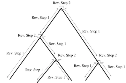
the upward and downward views just above that loca-tion, we show how we can obtain the upward views for each locus and for all the locations on the tree. (See Figure 4.)
The recursive formula has two parts, as was the case for the recursive formula in the section, a pruning algorithm. One part computes the upward view at the
bottom of a branch from the view at the location just below the top of the branch. We call this computational step reverse step 1. The other part of the formula computes the upward view at a location just below a node from the upward views at the node and the downward view for the other branch that is just below the node. We call this computational step reverse step 2.
Reverse step 1:In this section, we describe the
work-ings of reverse step 1. Consider a branch with bottom nodeyand top nodez. Assume that this branch comes to z from the left side. Let us recall that reverse step 1 computesC(y) fromC(L)(z) and the length of the branch,
CðyÞij ¼Prðry¼j;syðaÞjny¼iÞ
¼X
i
i9¼1
X
minði9;jÞ
j9¼maxð0;i9i1jÞ
Prðry¼j jrzðLÞ¼j9;s
ðaÞ
y ;n
ðLÞ
z ¼i9;ny¼iÞ
3PrðrðLÞ
z ¼j9;s
ðaÞ
y ;jn
ðLÞ
z ¼i9ÞPrðn
ðLÞ
z ¼i9jny¼iÞ
¼X
i
i9¼1
X
minði9;jÞ
j9¼maxð0;i9i1jÞ
Prðry¼jjrzðLÞ¼j9;n
ðLÞ
z ¼i9;ny¼iÞ
3CðLÞðzÞi9j9Qii9; ð8Þ
where the bounds oni9andj9come from the following relations:
0#rzðLÞ#ry; 0#nzðLÞr
ðLÞ
z #nyry; 1#nzðLÞ:
Combining (3) and (8), we have the required method for computingC(y).
Reverse step 2:Consider a nodex. Just below a nodex
in the branch coming from the left side, reverse step 2 computes C(L)(x) fromC(x),A(R)(x), andB(R)(x). Here
we give formula for the computation ofC(L)(x):
Figure4.—Flow of the computation using the two reverse
CðLÞðxÞij ¼PrðrðLÞ
x ¼j;s
ða;LÞ
x ;jn
ðLÞ
x ¼iÞ
¼PrðrðLÞ
x ¼j;s
ðb;RÞ
x ;s
ðaÞ
x jn
ðLÞ
x ¼iÞ
¼X
mxðbÞ
i9¼i
X
i9ðijÞ
j9¼j
Prðsðb;RÞ
x jrx¼j9;rxðLÞ¼j;s
ðaÞ
x ;nx¼i9;
nxðLÞ¼iÞ
3PrðrðLÞ
x ¼jjrx¼j9;sxðaÞ;nx ¼i9;nxðLÞ¼iÞ
3Prðrx¼j9;sðxaÞjnx¼i9ÞPrðnx¼i9jnðxLÞ¼iÞ
¼X
mxðbÞ
i9¼i
X
i9ðijÞ
j9¼j
Prðsðb;RÞ
x jr
ðRÞ
x ¼j9j;n
ðRÞ
x ¼i9iÞ
3PrðrðLÞ
x ¼jjrx¼j9;nx¼i9;nxðLÞ¼iÞ
3CðxÞi9j9PrðnxðRÞ¼ii9Þ
¼X
mxðbÞ
i9¼i
X
i9ðijÞ
j9¼j
BðRÞðxÞðii9Þðjj9ÞCðxÞi9j9A ðRÞðxÞ
ðiiÞ9
3PrðrðLÞ
x ¼jr
ðRÞ
x ¼jj9jrx¼j9;nx¼i9;
nðxLÞ¼iÞ;
ð9Þ
where the bounds oni9andj9come from the following relations:
rxðLÞ#rx; nxðLÞr
ðLÞ
x #nxrx; nxðLÞ#nx#mðxbÞ:
Combining (6) and (9), we have the formula forC(L)(x).
The computation ofC(R)(x) is analogous.
Maximization: We maximize the likelihood with
re-spect to the branch lengths for eachuin a grid of values ofu. For each value ofu, we maximize the likelihood with respect to one branch length and do this succes-sively for each branch in the tree. For each branch we carry out a simple line search over values separated by a constant small spacing. We repeat the process, continu-ing until none of the branches changes in a pass through the tree. After we have maximized the likeli-hood for the length of a branch, if the new length is different from its previous length, we recompute all views that are affected by that change of length. Once the maximization is done for each value ofu, we compare those maximum values and pick the overall maximum.
As we are searching over a grid of fixed spacing, the maximization takes a finite number of iterations. We have no proof that this process does not yield a local maximum within a topology and that another maxi-mum with a larger likelihood does not exist. However, we have not come across any data set where we have found two separate maxima within a topology.
This process maximizes the likelihood over branch lengths for a specified tree topology. The search for the maximum-likelihood tree involves either consideration of all possible tree topologies or heuristic searches that consider only neighboring tree topologies. For trees of
moderate to large size, exhaustive consideration of all topologies is not possible. The issues and strategies involved are the same as with other phylogeny inference problems. They are not described here. Common strategies are described by Felsenstein(2004, Chaps.
4 and 5).
SIMULATION STUDIES
To test the performance of our method, we carried out two simulation studies, one with four populations (repeated 10 times) and one with seven populations. A molecular clock is not assumed in any of these studies.
To simulate a data set from a completely specified tree, we start with simulatingL(number of loci) beta(u,
u) variables: p1;p2;. . .;pL. An array of N (population
size) Bernoulli(pl) variables are generated for each
pl;l ¼1;2;. . .;L. Then according to the structure of
the tree, the population is divided into two groups at each node and made to evolve according to a continu-ous-time Moran model at each branch (by having events that consist of selecting an individual to replace another individual, independently for each locus). At each branch the population is made to evolve the exact amount of time so that the scaled time passed at that branch agrees with the length of the corresponding branch of the tree. When the populations reach at the tip of the tree, we take a sample ofn individuals from each population; the data consist of the counts of 1 alleles at theLloci of all present-day populations.
In the first study the data consist of allele counts in 50 haploids from each population for 50 independent SNP loci. The data are simulated as described in the previous paragraph from a symmetric tree where the length of each branch is 0.02 and the value ofuis 0.05. Then the maximum-likelihood estimate (MLE) tree is estimated using our pruning algorithm. The same exercise is repeated 10 times, each time simulating the data in-dependently with the same parameters. Each time the true tree was estimated by our method. The estimated bias of the branch lengths is close to 0.005 for each branch.
In the second study, we tested our pruning algorithm in a tree with seven populations; the data consist of allele counts in eight haploids from each population for 500 independent SNP loci.
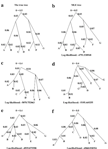
Note that there are.10,000 possible topologies for a seven-population tree. We have computed only the likelihood of the true topology and the other topologies that are nearest neighbors to the true topology.
In all cases that have misspecified topologies, the internal branches collapse to make the topology as close as to the topology of Figure 5a as possible. For example, when the branch adjacent to ‘‘G’’ of Figure 5b is reattached at the branch that is at the immediate right of the root, the tree of Figure 5c is the maximum-likelihood tree for the resulting topology. The internal branch created between the top of the branch adjacent to G and the meeting point of ‘‘E’’ and ‘‘F’’ collapses. (We do not have any proof that this will always be true; it is quite possible that for some data sets there may be local maxima of the likelihood for nonzero branch lengths within two or more tree topologies.)
Thus we have demonstrated that the correct topology can be estimated using our method. We saw no sign of systematic bias in the tree topology of branch lengths.
INFORMATION ABOUT THE ROOT
As mentioned in the Introduction, it is possible to estimate the root of the tree owing to the nonreversi-bility of the model. Here we investigate how much information a single locus provides for the estimation of the location of the root.
For simplicity we investigate the information on the location of the root in a tree with two populations. There is only one possible topology for a tree of two populations. The branch lengths determine the
loca-tion of the root. As the branch lengths are time scaled by effective population sizes, the ratio of the lengths of the branches is determined by the (unknown) ratio of the effective population sizes of the branches. So, the length of each branch can be treated as a free parameter.
A tree of two populations can be completely charac-terized by the total length of the two branches and the location of the root. To isolate the information about the root from the information about the total length of the two branches, we assume that we are aware of the total length (tt¼t11t2) of the two branches, but that the lengths (t1andt2) of the individual branches are unknown. In other words, we assume that we do not know the location of the root in an otherwise completely specified tree with two populations. The information about the root is obtained as
IrootðttÞ ¼E @logðLðt;tttÞÞ
@t
2
; ð10Þ
where L(., .) denotes the likelihood of a tree with two tips with the two branch lengths as the two arguments. The derivative of the likelihood in (10) is computed theoret-ically for all possible sets of allele counts. Then the expectation of the squared derivative of the likelihood is computed numerically. The likelihood is a weighted aver-age of the squared derivative over all possible data out-comes, weighted by the probability of each data outcome. Figure 6 plots the log10of the information about the root for different branch lengths in a tree with two tips. In each case, the information is for samples of size 10 from each tip. Figure 6 shows that the information is at a minimum at t1 ¼t2¼12ðt11t2Þ. If t1 6¼ t2, one population (Pop. 1) will be expected to have more extreme allele counts than the other (Pop. 2). Having more extreme allele counts indicates that Pop. 1 has the smaller population size of the two. Having a smaller
Figure 5.—Results from the simulation study with seven
populations.
Figure 6.—Information about the root from samples of
population size indicates that the length of the branch connected to Pop. 1 is bigger than that of Pop. 2. In other words, the root is closer to Pop. 2 than to Pop. 1. As demonstrated in Figure 6, the log10 of the information about the root ranges between 3 and 8 from the cases that we analyzed here. This suggests that the standard error of estimation of the root is at most of order 101.
IMPLEMENTING AN ASCERTAINMENT CORRECTION
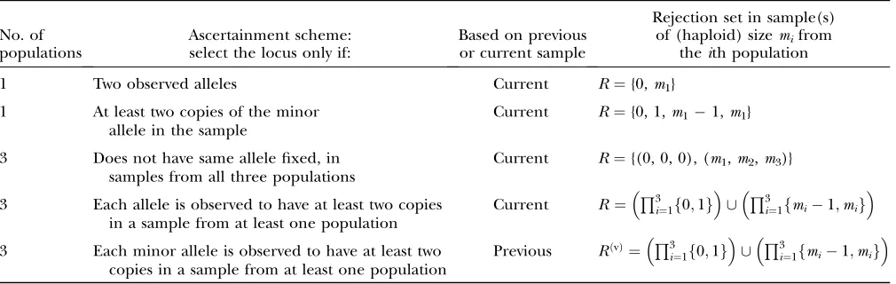
We can characterize the process of choice of SNPs by considering which loci will fail to be ascertained, as follows. If the observation from a locus falls into a predefined rejection set, then that locus will be ex-cluded from study. As a simple example, let us consider a sample of diallelic SNP loci. If we want to exclude those loci that have only one allele type in a sample of haploid sizem, our rejection set would be {0,m}. Table 2 shows examples of several possible ascertainment methods in one or more populations.
Ascertainment based on the current sample:
Ascer-tainment is sometimes based on the observations in the sample under study [for example, in The SNP Consor-tium study (Thorissonand Stein2003)]. In such cases,
we implement an ascertainment bias correction as follows.
Let the data be
D¼ fD1;D2;. . .;DPg;
from theP populations under study. Let the rejection set beR. Then, the ascertainment-corrected likelihood for the branch length vectortis given by
LðtjDÞ ¼PrðDjt;D;RÞ ¼ PrðDjtÞ
PrðD;RjtÞ:
Here, PrðDjtÞ is the same as the uncorrected likeli-hood. For the denominator, we need a mechanism of computing the collective probability of a set of possible
observations, rather than an individual observation. One way of doing this is to compute the probability of all the individual members of the set, and sum up. We will describe a more efficient computational method than this in an upcoming publication (A. RoyChoudhury
and E. A. Thompson, unpublished data).
Ascertainment based on a previous sample:In some
studies, ascertainment is done on the basis of data from a panel of SNPs (see, for example, Clarket al.2005). To
correct the bias induced by such ascertainments, we implement the following procedure.
Let us denote the data from the preliminary sample as
DðvÞ¼ fD1ðvÞ;Dð2vÞ;. . .;D ðvÞ
P g
and the rejection set in the preliminary sample asR(v).
Then, if D(v) is available for current analysis, the
ascertainment-corrected likelihood for the branch length vectortis given by
LðtjD;DðvÞÞ
¼PrðD;DðvÞjt;DðvÞ;RðvÞÞ ¼ PrðD
;DðvÞjtÞ PrðDðvÞ
;RðvÞjtÞ :
Here, PrðD;DðvÞjtÞ
is the uncorrected likelihood for the collection ofDandD(v). The denominator requires a
method for computing the probability of a collective set of possible observations. An efficient way of doing this will be demonstrated in an upcoming publication by A. RoyChoudhuryand E. A. Thompson(unpublished
data).
DISCUSSION
From the simulation studies, it is apparent that our method performs well. The branch length estimates were found to have a low bias. We must note that the first study is based on 50 loci only. In practice, there are thousands of independent SNP loci available in hu-mans. Conditional on the validity of the model, this
TABLE 2
Ascertainment schemes and their associated rejection sets
No. of populations
Ascertainment scheme: select the locus only if:
Based on previous or current sample
Rejection set in sample(s) of (haploid) sizemifrom
theith population
1 Two observed alleles Current R¼{0,m1}
1 At least two copies of the minor
allele in the sample
Current R¼{0, 1,m11,m1}
3 Does not have same allele fixed, in
samples from all three populations
Current R¼{(0, 0, 0), (m1,m2,m3)}
3 Each allele is observed to have at least two copies in a sample from at least one population
Current R¼Q3i¼1f0;1g[ Q3i¼1fmi1;mig
3 Each minor allele is observed to have at least two copies in a sample from at least one population
Previous RðvÞ¼ Q3
i¼1f0;1g
[ Q3i¼1fmi1;mig
large number of loci will give us much more accurate estimation of branch lengths using genomewide data.
The work in this article is an improvement on existing methods of exact-likelihood computation of a popula-tion tree using a coalescent model. It adds a manageable structure to the computation, resulting in increased tractability. Further, this method is free from use of any Monte Carlo technique and, as a result, can make a precise estimate without an indefinitely long run.
The difference in log-likelihood between competing topologies suggests that the data provide a wealth of information. We believe that this methodology will prove useful in analyzing data on polymorphisms across sub-species and populations. In theory, this method of pruning is applicable to data from loci with any number of alleles. However, the computational load of the pruning algorithm applied to a multiallelic loci could be very large. As we have to compute the probability of data conditional on all possible configurations of all the alleles at the root, the complexity will be of ordero(mk
), wherekis the total number of alleles andmis the total number of samples.
Although this is a significant improvement in com-puting the likelihood of a fully specified tree, the number of possible topologies makes maximum-likeli-hood estimation a daunting task for larger trees (.10 populations). With other kinds of data the problem of searching among tree topologies is also difficult, with some methods provably NP hard (Fouldsand Graham
1982; Grahamand Foulds1982).
The maximization is done as a line search over a fixed grid. We did not use a more sophisticated method for two reasons. The first reason is that some of the more sophisticated methods are not designed for optimizing multimodal functions. It is possible that our likelihood function is multimodal as the lengths of different branch may have similar effects on likelihood. There-fore we stick to grid search. The second reason is that grid search makes the computing simpler.
We have written a software based on our method. Using this software, the likelihood for the first study (four populations) took27 sec per locus to compute in a computer with 3 GHz CPU. For the second study (seven populations) it took,1 sec per locus in the same computer. The computation time can be drastically improved by efficient coding. We plan to recode parts of the software to make it more time efficient and make it available online.
We thank Matthew Stephens, Marco Bink, and an anonymous reviewer for their helpful comments. This work was supported in part
by National Institutes of Health (NIH) program project grant GM-45344, NIH program project grant GM 32544-14S1, and NIH grant R01 GM071639-01A1.
LITERATURE CITED
Cavalli-Sforza, L. L., and A. W. F. Edwards, 1967 Phylogenetic analysis. Models and estimation procedures. Am. J. Hum. Genet.
19:233–257.
Clark, A. G., M. J. Hubisz, C. D. Bustamante, S. H. Williamsonand R. Nielsen, 2005 Ascertainment bias in studies of human ge-nome-wide polymorphism. Genome Res.15:1496–1502. Edwards, A. W. F., and L. L. Cavalli-Sforza, 1964 Reconstruction
of evolutionary trees in phenetic and phylogenetic classifications. Syst. Assoc. Publ.6:67–76.
Elston, R. C., and J. Stewart, 1971 A general model for the anal-ysis of pedigree data. Hum. Hered.21:523–542.
Felsenstein, J., 1968 Statistical Inference and the Estimation of
Phylog-enies.Ph.D. Thesis, University of Chicago, Chicago.
Felsenstein, J., 1973a Maximum likelihood and minimum-steps methods for estimating evolutionary trees from data on discrete characters. Syst. Zool.22:240–249.
Felsenstein, J., 1973b Maximum-likelihood estimation of evolu-tionary trees from continuous characters. Am. J. Hum. Genet.
25:471–492.
Felsenstein, J., 1981 Evolutionary trees from DNA sequences: a maximum likelihood approach. J. Mol. Evol.17:368–376. Felsenstein, J., 2004 Inferring Phylogenies.Sinauer Associates,
Sun-derland, MA.
Foulds, L. R., and R. L. Graham, 1982 The Steiner problem in phy-logeny is np-complete. Adv. Appl. Math.3:43–49.
Graham, R. L., and L. R. Foulds, 1982 Unlikelihood that minimum phylogenies for a realistic biological study can be con-structed in reasonable computational time. Math. Biosci. 60:
133–142.
Heuch, I., and F. M. H. Li, 1972 PEDIG—a computer program for calculation of genotype probabilities, using phenotypic informa-tion. Clin. Genet.3:501–504.
Hilden, J., 1970 GENEX—an algebraic approach to pedigree prob-ability calculus. Clin. Genet.1:319–348.
Moran, P. A. P., 1962 The Statistical Processes of Evolutionary Theory. Clarendon Press, Oxford.
Nielsen, R., and M. Slatkin, 2000 Likelihood analysis of ongoing gene flow and historical association. Evolution54:44–50. Nielsen, R., J. L. Mountain, J. P. Huelsenbeckand M. Slatkin,
1998 Maximum likelihood estimation of population diver-gence times and population phylogeny in models without muta-tion. Evolution52:669–677.
Takahata, N., and M. Nei, 1985 Gene genealogy and variance of interpopulational nucleotide differences. Genetics 110:
325–344.
Thompson, E. A., 1975 Human Evolutionary Trees.Cambridge Univer-sity Press, Cambridge, UK.
Thorisson, G. A., and L. D. Stein, 2003 The SNP Consortium web-site: past, present and future. Nucleic Acids Res.31:124–127. Wright, S., 1931 Evolution in Mendelian populations. Genetics16:
97–159.