1
Modeling and forecasting Daily stock Returns of Guaranty Trust
Bank Nigeria Plc Using ARMA-GARCH Models, Persistence, Half-life
Volatility and Backtesting
1
Emenogu, G. Ngozi;
2*
Adenomon, Monday Osagie &
2
Nweze, Nwaze Obinna
1. Department of Statistics, Federal Polytechnic, Bida, Niger State, Nigeria
2. Department of Statistics, Nasarawa State University, Keffi, Nasarawa State, Nigeria
* Corresponding Authors: [email protected]; [email protected];
[email protected] +2347036990145; +2348036759112
Abstract
In financial time series modelling and forecasting, combining ARMA and GARCH models tend
to produce superior and reliable models for volatility persistence, half-life volatility and
backtesting (application of model in real life). In Nigeria, banking stocks are mostly traded
because of its potential benefits to investors. This study modelled and forecasted the Guaranty
Trust (GT) Bank daily stock returns from January 2
nd
2001 to May 8
th
2017 data set collected
from a secondary source. The ARMA-GARCH models, persistence, half-life and backtesting
were used to analysed the collected data using student t and skewed student t distributions, and
the analyses are carried out R environment using rugard and performanceAnaytics Packages. The
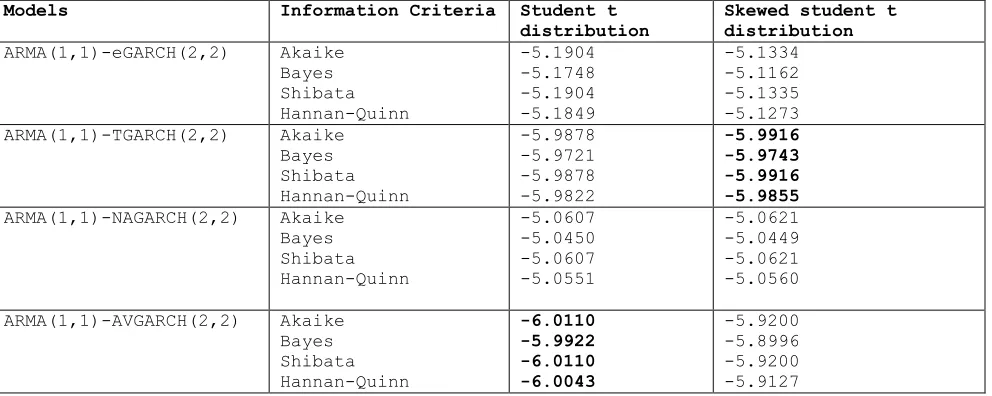
study revealed that using the lowest information criteria values only could be misleading rather
we added the use of backtesing. The ARMA(1,1)-GARCH(1,1) models fitted exhibited high
persistency in the daily stock returns while the days it takes for mean-reverting of the models
ranges from 5 days to 100 days but unfortunately the models failed backtesting. The results
further revealed ARMA(1,1)-eGARCH (2,2) model with student t distribution provides a
suitable model for evaluating the GT bank stock returns among the competing models while it
takes less than 30 days for the persistence volatility to return back to its average value of the
stock returns. This study recommended that researchers should adopt backtesting approach while
fitting GARCH models while GT bank stocks investor should be assured that no matter the
fluctuations in the stock market, the GT bank stock returns has the ability to returns to its mean
price return.
Keywords: Returns, Stocks, Guaranty Trust (GT) Bank, Generalized Autoregressive Conditional
Heteroskedasticity (GARCH), Persistence, Half-life, Volatility, Backtesting.
2
1.0
Introduction
Autoregressive Moving Average (ARMA) and Autoregressive Integrated Moving Average
(ARIMA) models are popular and excellent for modeling and forecasting univariate time series
data as proposed by Box and Jenkins (1970), and its extension with exogenous variables as
Autoregressive Integrated Moving Average with Explanatory Variable (ARIMAX)
(Kongcharoen and Kruangpradit, 2013). These models are applied in almost all fields of
endeavours such as engineering, geophysics, business, economics, finance, agriculture, medical
sciences, social sciences, meteorology, quality control etc (Kirchgassner and Wolters, 2007;
Adenomon, 2017a, Adenomon, 2017b; Cooray, 2008; Dobre and Alexandru, 2008; Gujarati,
2003; Adekeye and Aiyelabegan, 2006). The ARMA and ARIMA models are used to model
conditional expectation of a process but in ARMA model, the conditional variance is constant.
This means that ARMA model cannot capture process with time-varying conditional variance
(volatility) which is mostly common with economic and financial data.
Actually, with economic and financial time series data, time-varying is more common
than constant volatility, and accurate modeling of time volatility is of great importance in
financial time series analysis (Ruppert, 2011). Financial time series contains uncertainty,
volatility, excess kurtosis, high standard deviation, high skewness and sometimes non normality
(Pedroni (2001); Grigoletto & Lisi (2009); Emenogu and Adenomon, 2018; Emenogu et al.
2018). To model and capture properly the characteristics of financial time series models such as
Auto-Regressive
Conditional
Heteroscedastic
(ARCH),
Generalized
Auto-Regressive
Conditional Heteroscedastic (GARCH), multivariate GARCH, Stochastic volatitlity (SV) and
various variants of the models have been proposed to handle these characteristics of financial
time series (Lawrance, 2003).
3
take a better decision. This paper therefore investigates the persistence, half-life volatility and
forecasting (Backtesting that is providing real life model) of daily stock returns of Guaranty
Trust Bank, Nigeria plc using ARMA-GARCH Models.
Guaranty Trust (GT) Bank plc was incorporated as a limited liability company licensed to
provide commercial and other banking services to the Nigerian public in 1990. The Bank
commenced operations in February 1991, and has since then grown to become one of the most
respected and service focused banks in Nigeria. Also, In September 1996, Guaranty Trust Bank
plc became a publicly quoted company and won the Nigerian Stock Exchange President’s Merit
award that same year, and subsequently in the years 2000, 2003, 2005, 2006, 2007, 2008 and
2009. In February 2002, the Bank was granted a universal banking license and later appointed a
settlement bank by the Central Bank of Nigeria (CBN) in 2003. In May 2011, The Bank
successfully launched a US$500 million bond — which bring about the first non-sovereign
benchmark bond offering from sub-Saharan Africa (outside South Africa), to the international
community. The highly successful offering, which matures in 2016, went further to show that the
international finance community’s believe in the GT Bank brand. The Bank’s culture is tied to
eight guiding principles called the Orange Rules; Simplicity, Professionalism, Service,
Friendliness, Excellence, Trustworthiness, Social Responsibility and Innovation. With these
features of GT Bank, the bank stands suitable for customers and investor both in Nigeria and
abroad where the bank has branches (The European Financial Review, 2012).
2.0
Brief literature on the persistence and half-life Volatility of Stocks Returns
The volatility of asset returns is a measure of how much the returns fluctuates around its
means (Marra, 2015). In addition, volatility is the purest measure of risk in financial markets and
by this, it has becomes the expected price of uncertainty. A good volatility model and forecast
help impact the public confidence significantly and by extension on the broader global economy.
What comes to mind again is the persistence and half-life volatility of any given stock.
4
financial time series it is usually close to one (1) (Ahmed et al., 2018; Engle and Patton, 2001;
Vosvrda, 2006). While on the other hand, the half-life of the volatility shocks measure the
average time period for the volatility to return back to it mean value in the long run horizon
(Ahmed et al., 2018; Sahai, 2016).
Engle and Patton (2001) examine the Dow Jones Industrial index from 23 August 1988 to
22 August 2000. Their result indicated that the volatility returns are quite persistent.
Magnus and Fosu (2006) modeled and forecasted the volatility of returns on Ghana Stock
exchange using GARCH models. They found that presence of high level of persistence in the
returns in the stock market.
Vosvrda (2006) compared empirical analysis of persistence and dependence patterns
among capital market using univariate and multivariate measures. The results revealed that the
univariate measure shows a low level of persistence while multivariate measure shows that the
persistence change dependence on structure in different period of lags.
Panait and Slavescus (2012) investigated the volatility and persistence of seven
Romanian companies traded on Bucharest Stock Exchange and three market indices from
1997-2012 using GARCH-in-Mean Models. They found out that persistency is more in the daily
returns as compared to weekly and monthly series.
Emenike and Ani (2014) examined the nature of volatility of stock returns in the Nigerian
banking sector using ARMA-GARCH models using data covering 3
rd
January to December
2012. Their results revealed volatility persistence was high for the sample period they
considered.
Usman et al. (2017) examined the performance of eleven competing GARCH models for
fitting the rate of returns of monthly observations on the index returns series of the market over a
period of January 1996 to December 2015. The overall results revealed increased volatility of the
market returns.
5
Kuhe (2018) examined the volatility persistence and asymmetry with exogenous break in
Nigerian stock market using data from 3
rd
July 1999 to 12
th
June 2017 using standard symmetric
GARCH (1,1), asymmetric EGARCH (1,1) and GJR-GARCH (1,1) models. The study revealed
among other results a high persistence of shocks in the return series for the estimated models.
Ahmed et al. (2018) examined and compared the mean reversion phenomenon in
developed and emerging stock markets, they employed data from 1
st
January to 30
th
June 2016
using GARCH (1,1) model. There results revealed that South Korean market has the slowest
mean reversion and thus has the highest half-life period while Pakistan stock exhibited fastest
reverting process.
3.0
Model Specification
This study focuses on the ARMA-GARCH models that are robust for forecasting the
volatility of financial time series data; so ARMA-GARCH model and some of its extensions are
presented in this section.
ARMA-GARCH specification is employed to model the conditional mean and
conditional variance (volatility) of any financial time series because of its superiority in
modelling such series. GARCH models model conditional variances much as the conditional
expectation by an ARMA model (Ruppert, 2011). Therefore ARMA model can be combined to
any form of GARCH model.
The ARMA (p,q)-GARCH (1,1) model can be specified as follows:
(1)
)
D(0,
~
,
2 1 -t 1 2
1 -t 1 2
t
2 t 2
1
+
+
=
+
+
=
−
−=
t t
t t
q
j
t j t j i
t p
i i t
Z
Z
r
r
Where r
t
is the daily rate of return,
is the AR(p) term in the mean equation in order to account
for time dependence in returns,
is the MA(q) term in the mean equation,
tis the residual term
in the mean equation, Z
t
is the standardized residual sequence of iid random variable with mean
6
Because of space we will discussion the follow family GARCH models below:
3.1
Autoregressive Conditional Heteroskedasticity (ARCH) Family Model
Every ARCH or GARCH family model requires two distinct specifications, namely: the mean
and the variance equations (Atoi, 2014). The mean equation for a conditional heteroskedasticity
in a return series,
y
tis given by
t t t
t
E
y
y
=
−1(
)
+
(2)
where
t=
t
tThe mean equation in equation (2) also applies to other GARCH family models.
E
t−1(.)
is the
expected value conditional on information available at time
t-1
, while
tis the error generated
from the mean equation at time t and
tis the sequence of independent and identically
distributed random variables with zero mean and unit variance.
The variance equation for an ARCH(p) model is given by
2 2
1 1 2
...
p t pt
t
=
+
a
−+
+
a
−
(3)
It can be seen in the equation that large values of the innovation of asset returns have bigger
impact on the conditional variance because they are squared, which means that a large shock
tends to follow another large shock and that is the same way the clusters of the volatility behave.
So the ARCH(p) model becomes:
a
t=
t
t,
t2=
+
1a
t2−1+
...
+
pa
t2−p(4)
Where
t~
N
(0,1)
iid
,
> 0 and
i
0
for
i
> 0. In practice,
tis assumed to follow the
standard normal or a standardized student-
t
distribution or a generalized error distribution (Tsay
2005).
3.2
Asymmetric Power ARCH
According to Rossi (2004), the asymmetric power ARCH model proposed by Ding, Engle &
Granger (1993) given below forms the basis for deriving the GARCH family models
Given that:
t
a
r
=
+
,
t t t
=
,
)
1
,
0
(
~
N
t
7
= −
= − −
+
−
+
=
qj
j t j p
i
i t i i t i
t
a
a
1 1
)
(
,
(5)
where
0
,
0
,
0
i
i
=
1
,
2
,
,
p
1
1
−
ii
=
1
,
2
,
,
p
0
j
j
=
1
,
2
,
,
q
This model imposes a Box-Cox transformation of the conditional standard deviation process and
the asymmetric absolute residuals. The leverage effect is the asymmetric response of volatility to
positive and negative “shocks”.
3.3
Standard GARCH(p, q) Model:
The mathematical model for the sGARCH(p,q) model is obtained from equation (5) by letting
2
=
and
i=
0
,
i
=
1
,
,
p
to be:
t t t
a
=
,
= − = −
+
+
=
pi
q
j
j t j i
t i
t
a
1 1
2 2
2
(6)
Where
a
t=
r
t−
t(
r
tis the continuously compounded log return series), and
t
~
N
(0,1)
iid
, the parameter
iis the ARCH parameter and
jis the GARCH parameter, and
> 0,
i0,
j0, and
=+
) , max(1
(
)
q p
i
i
i< 1, (Rossi, 2004; Tsay, 2005 and Jiang, 2012).
The restriction on ARCH and GARCH parameters
(
i,
j)
suggests that the volatility (
a
i) is
finite and that the conditional standard deviation (
i) increases. It can be observed that if q = 0,
then the model GARCH parameter (
j) becomes extinct and what is left is an ARCH(p) model.
To expatiate on the properties of GARCH models, the following representation is necessary:
Let
t=
a
t2−
t2so that
t=
a
t−
t2 2
. By substituting
t−i=
a
t−i−
t−i 2 2, (
i
= 0
, . . . , q
) into Eq.
(4), the GARCH model can be rewritten as
t
a
=
= −
= −
−
+
+
+
qj
j t j t
q p
i
i t i
i
a
1 )
, max(
1
2
0
(
)
,
(7)
8
0
)
,
cov(
t
t−j=
, for
j
≥ 1). However, {
t} in general is not an iid sequence.
A GARCH model can be regarded as an application of the ARMA idea to the squared series
a
t2.
Using the unconditional mean of an ARMA model, results in this
E(
a
t2) =
=+
−
max( , )1 0
)
(
1
pqi
i
i
provided that the denominator of the prior fraction is positive. (Tsay, 2005)
When p =1 and q =1, we have GARCH(1, 1) model given by:
t t t
a
=
,
2 1 1 2 1 1 2 − −+
+
=
t tt
a
,
(8)
3.4
GJR-GARCH(p, q) Model
The Glosten-Jagannathan-Runkle GARCH (GJRGARCH) model, which is a model that attempts
to address volatility clustering in an innovation process, is obtained by letting
=
2
.
When
=
2
and
0
i
1
,
= − − = −+
−
+
=
p i q j j t j i t i i t i t 1 1 2 2 2)
(
(9)
=
= − − − − = −+
−
+
+
p i q j j t j i t i t i t i i t i 1 1 2 2 1 2 2)
2
(
+
−
+
+
+
+
=
= − = − − = − = − − p i q j i t j t j i t i i p i q j i t j t j i t i i t 1 1 2 2 2 1 1 2 2 2 2 20
,
)
1
(
0
,
)
1
(
i.e;
= = − = − − −
+
+
−
−
+
−
+
=
p i q j j t j p i i t i i i i i t i i tS
1 1 2 1 2 2 2 2 2 2}
)
1
(
)
1
{(
)
1
(
2 1 1 2 1 2 1 1 2 24
)
1
(
i i t ip i i q j t j t p i i i
t
S
−9
2 *)
1
(
i ii
=
−
and
i*=
4
i
i,
then
= − − = − = −+
+
−
+
=
q j t i p i i i t j p i i t i i tS
1 2 1 1 * 2 1 2 2 2)
1
(
(10)
Which is the GJRGARCH model (Rossi, 2004).
But when
−
1
i
0
,
Then recall Eq. (9)
= − − = −+
−
+
=
p i q j j t j i t i i t i t 1 1 2 2 2)
(
=
= − − − − = −+
−
+
+
p i q j j t j i t i t i t i i t i 1 1 2 2 1 2 2)
2
(
+
+
+
+
−
+
=
= − = − − = − = − − p i q j i t j t j i t i i p i q j i t j t j i t i i t 1 1 2 2 2 1 1 2 2 2 2 20
,
)
1
(
0
,
)
1
(
= = − + = − −+
+
−
−
+
+
+
=
p i p i i t i i i i q j j t j i t i i tS
1 1 2 2 2 1 2 2 2 2}
)
1
(
)
1
{(
)
1
(
= = − + = − −+
+
+
−
−
−
−
+
+
=
p i p i i t i i i i i i q j j t j i t i iS
1 1 2 2 2 1 2 2 2}
2
1
2
1
{
)
1
(
Where
=
− − +0
if
0
0
if
1
i t i t iS
also define
2 *)
1
(
i ii
=
+
and
i4
i
i*
=
−
,
then
= − + = − = −+
+
+
=
q j t i p i i i t j p i i t i tS
1 2 1 1 * 2 1 2 *2
(11)
10
2 1 2
1 2
2
− −
+
+
+
=
t i t tt
S
.
(12)
3.5
IGARCH(1, 1) Model
The integrated GARCH (IGARCH) models are unit- root GARCH models. The IGARCH (1, 1)
model is specified in Tsay (2005) and Grek (2014) as
t t t
a
=
;
t2=
0+
1
t2−1+
(
1
−
1)
a
t2−1(13)
Where
t~ N(0, 1)
iid
, and
0
1
1
, Ali (2013) used
ito denote
1
−
i.
The model is also an exponential smoothing model for the {
a
t2} series. To see this, rewrite the
model as
2 t
=
1 212 1 1
)
1
(
−
a
t−+
t−=
(
1
−
1)
a
t2−1+
1[(
1
−
)
a
t2−2+
1
t2−2]
=
(
1
−
1)
a
t2−1+
(
1
−
1)
1a
t2−2+
12
t2−2.
(14)
By repeated substitutions, we have
)
)(
1
(
1 21 1 22 12 332
=
−
+
+
+
− −
− t t
t
t
a
a
a
,
(15)
which is the well-known exponential smoothing formation with
1being the discounting factor
(Tsay, 2005).
3.6
TGARCH(p, q) Model
The Threshold GARCH model is another model used to handle leverage effects, and a
TGARCH(p, q) model is given by the following:
= = − = −
+
+
+
=
pi
q
j
j t j i
t i t i i
t
N
a
1 1
2 2
0 2
)
(
,
(16)
where
N
t−iis an indicator for negative
a
t−i, that is,
i t
N
−=
− −
,
0
if
0
,
0
if
1
i t
i t
a
a
and
i,
i, and
jare nonnegative parameters satisfying conditions similar to those of GARCH
models, (Tsay, 2005). When
p
=
1
,
q
=
1
, the TGARCH(1, 1) model becomes:
2 1 2
1 1 2
)
(
+
− −+
−+
=
t t tt
N
a
11
3.7
NGARCH(p, q) Model
The Nonlinear Generalized Autoregressive Conditional Heteroskedasticity (NGARCH) Model
has been presented variously in literature by the following scholars: Hsieh & Ritchken (2005),
Lanne & Saikkonen (2005), Malecka (2014) and Kononovicius & Ruseckas (2015). The
following model can be shown to represent all the presentations:
= − = − = −+
+
+
=
q i q i p j j t j i t i i t i th
h
1 1 1
2
(18)
Where
h
tis the conditional variance, and
,
and
satisfy
0
,
0
and
0
.
Which can also be written as
= − = − = −+
+
+
=
q i q i p j j t j i t i i t i t1 1 1
2
(19)
3.8
The Exponential Generalized Autoregressive Conditional Heteroskedasticity
(EGARCH) Model
The EGARCH model was proposed by Nelson (1991) to overcome some weaknesses of the
GARCH model in handling financial time series pointed out by Enocksson and Skoog(2012), In
particular, to allow for asymmetric effects between positive and negative asset returns, he
considered the weighted innovation
)]
(
[
)
(
t t tE
tg
=
+
−
,
(20)
where
and
are real constants. Both
tand
t−
E
(
t)
are zero-mean iid sequences with
continuous distributions. Therefore,
E
[
g
(
t)]
=
0
. The asymmetry of
g
(
t)
can easily be seen by
rewriting it as
−
−
−
+
=
.
0
if
)
(
)
(
,
0
if
)
(
)
(
)
(
t t t t t t tE
E
g
(21)
An EGARCH(
m, s
) model, according to Tsay (2005), Dhamija and Bhalla (2010), Jiang (2012),
Ali (2013) and Grek (2014), can be written as
t t t
a
=
,
= − = − − −
+
+
+
=
s i m j i t j i t i t i i t i ta
a
1 1 2 2)
ln(
)
ln(
,
(22)
12
t t t
a
=
(
)
)
ln(
)
(
)
ln(
t2=
+
a
t−1−
E
a
t−1+
a
t−1+
t2−1(23)
where
a
t−1−
E
(
a
t−1)
are
iid
and have mean zero. When the EGARCH model has a Gaussian
distribution of error term, then
E
(
t)
=
2
/
, which gives:
2
/
)
ln(
)
(
)
ln(
t2=
+
a
t−1−
+
a
t−1+
t2−1(24)
3.9
The Absolute Value GARCH (AVGARCH):
An asymmetric GARCH (AGARCH), according to Ali (2013) is simply
a
t=
t
t;
= − = −
+
−
+
=
q j j t j p i i t ib
1 2 1 22
,
(25)
While the absolute value generalized autoregressive conditional heteroskedasticity (AVGARCH)
model is specified as:
t t t
a
=
;
= − − = −
+
+
−
+
+
=
q j j t j i t p i i ti
b
c
b
1 2 2 1 2
))
(
(
(26)
3.10
Nonlinear (Asymmetric) GARCH, or N(A)GARCH or NAGARCH
NAGARCH plays key role in option pricing with stochastic volatility because, as we shall see
later on, NAGARCH allows you to derive closed-form expressions for European option prices in
spite of the rich volatility dynamics. Because a NAGARCH may be written as
(27)
)
(
2 22 2
1 t t t
t
z
+=
+
−
+
And if
z
t~
IIDN
(
0
,
1
)
,
z
tis independent of
2 t
as
t2is only a function of an infinite number of
past squared returns, it is possible to easily derive the long run, unconditional variance under
NGARCH and the assumption of stationarity:
2 2 2 2 2 2 2 2 2 2 2 2 1
)
1
(
]
[
]
2
(
]
[
]
[
]
)
(
[
]
[
+
+
+
=
+
−
+
+
=
+
−
+
=
=
+ t t t t t t t tE
z
z
E
E
E
z
E
E
(28)
Where
2=
E
[
t2]
and
[
]
[
21]
2
+
=
tt
E
13
+
+
−
=
=
+
+
−
)
1
(
1
]
)
1
(
1
[
2 2 22
(29)
Which exists and positive if and only if
(
1
+
2)
+
1
. This has two implications:
(i)
The persistence index of a NAGARCH(1,1) is
(
1
+
2)
+
and not simply
+
;
(ii) a NAGARCH(1,1) model is stationary if and only if
(
1
+
2)
+
1
.
See details in Nelson (1991); Hall & Yao (2003); Enders (2004); Christo
ff
ersen, et al. (2008)
and Engle & Rangel (2008).
3.11
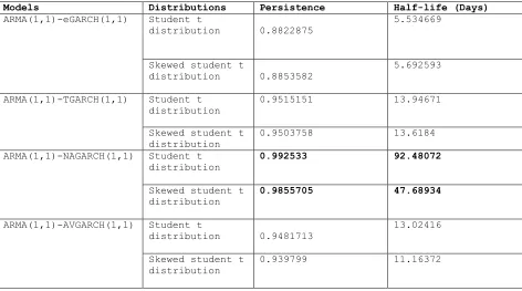
Persistence, Half-life Volatility and Backtesting
3.11.1 Persistence
The low or high persistency in volatility exhibited by financial time series can be
determined by the GARCH coefficients of a stationary GARCH model. The persistence of a
GARCH model can be calculated as the sum of GARCH (
1) and ARCH (
1) coefficients that
is
+
1. In most financial time series, it is very close to one (1) (Banerjee and Sarkar, 2006;
Ahmed et al, 2018). Persistence could take the following conditions:
If
+
1
1
: The model ensures positive conditional variance as well as stationary.
If
+
1=
1
: we have an exponential decay model, then the half-life becomes infinite. Meaning
the model is strictly stationary.
If
+
1
1
: The GARCH model is said to be non-stationary, meaning that the volatility
ultimately detonates toward the infinitude (Ahmed et al, 2018). In addition, the model shows that
the conditional variance is unstable, unpredicted and the process is non-stationary (Kuhe, 2018).
3.11.2 Half-Life Volatility
Half-life volatility measures the mean reverting speed (average time) of a stock price or
returns. The mathematical expression of half-life volatility is given as
)
ln(
)
5
.
0
ln(
2 1
+
=
−
Life
Half
14
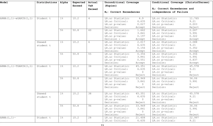
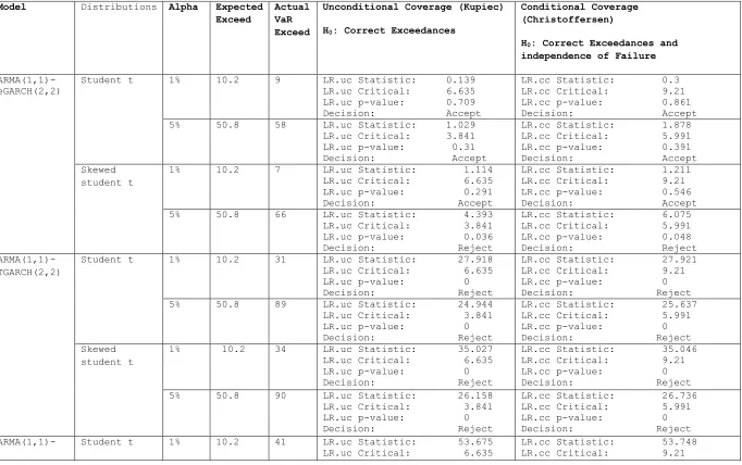
3.11.3 Backtesting
Financial risk model evaluation or backtesting is an important part of the internal model’s
approach to market risk management as put out by Basle Committee on Banking Supervision
(Christoffersen & Pelletier, 2004). Backtesting is a statistical procedure where actual profits and
losses are systematically compared to corresponding VaR estimates (Nieppola, 2009; Emenogu,
et al., 2018). This study adopted Backstesting techniques of Christoffersen & Pelletier, (2004);
The test was implemented in R using rugarch package and this test considered both the
unconditional (Kupiec) and conditional (Christoffersen) coverage tests for the correct number of
exceedances (see details in Christoffersen(1998) and Christoffersen et al. (2001)).
The unconditional (Kupiec) test also refer to as POF-test (Proportion of failure) with its null
hypothesis given as
T
y
p
p
H
0:
=
ˆ
=
Here y is the number of exceptions and T is the number of observations and k is the confidence
level. The test is given as
−
−
−
=
−− yT y y T p y
y y T POF
p
p
LR
)
(
)
(
1
[
)
1
(
ln
2
.
Under the null hypothesis that the model is correct and
LR
POFis asymptotically chi-squared
(
2) distributed with degree of freedom as one (1). If the value of the
LR
POFstatistic is greater
than the critical value (or p-value<0.01 for 1% level of significant or p-value<0.05 for 5% level
of significant) the null hypothesis is rejected and the model then is inaccurate.
The Christoffersen’s Interval Forecast Test combined the independence statistic with the
Kupiec’s POF test to obtained the joint test (Christoffersen, 1998; Nieppola, 2009). This test
examined the properties of a good VaR model, the correct failure rate and independence of
exceptions, that is condition coverage (cc). the conditional coverage (cc) is given as
ind POF
cc
LR
LR
LR
=
+
Where
−
−
−
−
−
−
=
−−= −
−
1 1 11
2
1 1 1
1
)
1
)(
(
)
1
(
ln
2
)
1
)(
(
)
1
(
ln
2
uu u
u n
i
u u u
u ind
p
p
p
p
LR
i
i i
15
Where
u
iis the time between exceptions I and i-1 while u is the sum of
u
iIf the value of the
LR
ccstatistic is greater than the critical value (or p-value<0.01 for 1% level of
significant or p-value<0.05 for 5% level of significant) the null hypothesis is rejected and that
leads to the rejection of the model.
3.12
Distributions of GARCH models
In this study we employed two innovations namely student t and skewed student t distributions
they can account for excess kurtosis and non-normality in financial returns (Heracleous, 2003;
Wilhelmsson, 2016; Kuhe, 2018).
The student t distribution is given as
−
+
=
+ − +y
v
y
f
v v y v v;
)
1
(
)
(
)
(
)
(
2 ) 1 ( 2 2 2 1
The Skewed student t distribution is given as
−
+
−
+
=
+ − + − − + + − − − + − b a a b v b a a b vy
if
bc
y
if
bc
v
y
f
v y v y,
1
,
1
)
,
,
,
;
(
2 1 2 1 2 1 ) ( 2 1 2 1 ) ( 2 1
Where
v
is the shape parameter with
2
v
and
is the skewness parameter with
−
1
1
.
The constants a, b and c are given as
)
(
)
2
(
)
(
;
)
(
3
1
;
1
2
4
2 2 1 2 2 v vv
c
a
b
v
v
c
a
−
=
−
+
=
−
−
=
+
Where
and
are the mean and the standard deviation of the skewed student t distribution
respectively.
4.0
Materials and Methods
The data used in this study was collected from
www.cashcraft.com
under stock trend and
analysis. Daily stock price for Guaranty Trust Bank Nigeria plc from January 2
nd
2001 to May 8
th
2017 (a total of 4017 observations) was collected from the website. The returns was calculated
using the formula below
1
ln
ln
−
−=
t tt
P
P
R
.
(30)
16
5.0
Results
The analyses of this study was carried in R environment using rugarch package by Ghalanos
(2018) and PerformanceAnalytics package by Peterson et al.(2018). The section begins with the
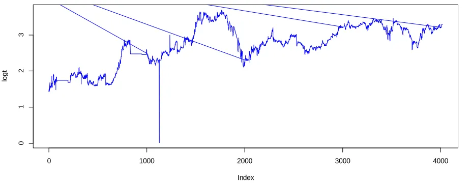
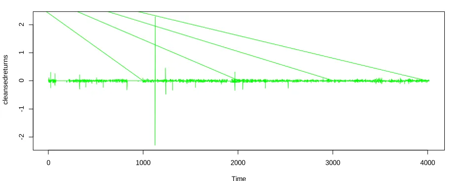
descriptive statistics of the daily stock price of GT Bank Nigeria, plc. Figures 1, 2, 3 and 4
presents the plot of the daily actual price of GT bank stock, the plot of the log Transform of the
actual price of GT bank stock, the plot of log transformed of stock returns of GT Bank daily
stock price and the plot of cleansed log transform of stock returns of GT Bank respectively.
Time
P
ri
ce
2000 3000 4000 5000 6000
0
10
20
30
40
Fig. 1: Plot of the Actual price of GT bank stock
17
0 1000 2000 3000 4000
0
1
2
3
Index
lo
g
t
Fig. 2: Plot of the log Transform of the Actual price of GT bank stock
Figure 2 above presents the log transform of the Actual price of the Guaranty Bank stock plc
from January 2
nd
2001 to May 8
th
2017. The figure exhibited some pattern and achieved stability
through transformation.
Time
G
T
B
a
n
k
0 1000 2000 3000 4000
-2
-1
0
1
2
Fig 3: Plot of log transformed of stock returns of GT Bank
18
Time
cl
e
a
n
se
d
re
tu
rn
s
0 1000 2000 3000 4000
-2
-1
0
1
2