Alternating direction implicit finite difference methods for a new two dimensional two sided space fractional diffusion equation

R E S E A R C H

Open Access

Alternating-direction implicit finite

difference methods for a new

two-dimensional two-sided space-fractional

diffusion equation

Xiucao Yin

_{, Shaomei Fang}

_{and Changhong Guo}

*_{Correspondence:}

[email protected]

2_{Department of Mathematics,}

South China Agricultural University, Guangzhou, China

Full list of author information is available at the end of the article

Abstract

According to the principle of conservation of mass and the fractional Fick’s law, a new two-sided space-fractional diffusion equation was obtained. In this paper, we present two accurate and efficient numerical methods to solve this equation. First we discuss the alternating-direction finite difference method with an implicit Euler method (ADI–implicit Euler method) to obtain an unconditionally stable first-order accurate finite difference method. Second, the other numerical method combines the ADI with a Crank–Nicolson method (ADI–CN method) and a Richardson extrapolation to obtain an unconditionally stable second-order accurate finite difference method. Finally, numerical solutions of two examples demonstrate the effectiveness of the theoretical analysis.

Keywords: Two-dimensional two-sided space-fractional diffusion equations; The shifted left Grünwald formula; The standard right Grünwald formula; ADI methods; Richardson extrapolation

1 Introduction

According to the principle of conservation of mass, the equation of continuity form is given by

∂u(x,t)

∂t +

∂Q(x,t)

∂x =f(x,t), (1.1)

whereu(x,t) is the distribution function of the diffusing quantity,Q(x,t) is the diffusion flux, andf(x,t) is the source term. Then we modified the classical Fick’s law by

Q(x,t) = –C(x) ∂

∂x

x

a

K+(x,ξ)u(ξ,t)dξ–D(x)

∂ ∂x

b

x

K–(x,ξ)u(ξ,t)dξ, (1.2)

whereC(x) andD(x) are nonnegative diffusion coefficients,K+(x,ξ) andK–(x,ξ) are the

kernel functions defined by

⎧ ⎨ ⎩

K+(x,ξ) =(1–1α)(x–ξ)

–α_{, a≤ξ≤x;}

K–(x,ξ) =_(1–1_α)(ξ–x)–α, x≤ξ≤b,

(1.3)

where 0 <α< 1. Combining Eqs. (1.1)–(1.3), we can get a one-dimensional two-sided space-fractional diffusions equation [1]:

∂u(x,t)

∂t =

∂ ∂x

C(x)∂

α_u(x,t)

∂xα –D(x)

∂α_u(x,t)

∂(–x)α

+f(x,t),

a≤x≤b, 0 <α< 1,t> 0. (1.4)

In this paper, we discuss the two-dimensional two-sided space-fractional diffusion equa-tion as follows:

∂u(x,y,t)

∂t =

∂ ∂x

Cx(x,y)

∂αu(x,y,t)

∂xα –Dx(x,y)

∂αu(x,y,t)

∂(–x)α

+ ∂

∂y

Cy(x,y)

∂β_u(x,y,t)

∂yβ –Dy(x,y)

∂β_u(x,y,t)

∂(–y)β

+f(x,y,t), (x,y)∈,t> 0, (1.5)

subject to the initial condition

u(x,y, 0) =φ(x,y), (x,y)∈ ¯, (1.6)

and the zero Dirichlet boundary conditions

u(a1,y,t) =u(a2,y,t) =u(x,b1,t) =u(x,b2,t) = 0, t≥0, (1.7)

where= (a1,a2)×(b1,b2) is a rectangular domain, 0 <α,β< 1,Cx(x,y),Dx(x,y),Cy(x,y), andDy(x,y) are the nonnegative diffusion coefficients,f(x,y,t) is the source term. The

∂γ_u(x,y,t)

∂xγ ,

∂γ_u(x,y,t)

∂(–x)γ (γ =α orβ) are respectively the left and right Riemann–Liouville frac-tional derivatives [2,3] which are defined by

∂γ_u(x,y,t)

∂xγ =

1

(1 –γ)

∂ ∂x

x

a1

u(s,y,t)

(x–s)γ ds, (1.8)

∂γu(x,y,t)

∂(–x)γ =

–1

(1 –γ)

∂ ∂x

a2

x

u(s,y,t)

(s–x)γ ds. (1.9)

The definitions of ∂γu_∂(_yxγ,y,t),

∂γu(x,y,t)

∂(–y)γ are similar to the definitions of thex direction. As we cannot easily get the explicit analytical solutions of the fractional equations, so many researchers resort to their numerical solutions [4–10].

proposed a Crank–Nicolson alternating-direction implicit Galerkin–Legendre spectral method for the two-dimensional Riesz space fractional nonlinear reaction-diffusion equa-tions. Feng et al. [16] presented a second-order method for the space fractional diffusion equation with variable coefficient. Moroney et al. [17] developed a fast Poisson precondi-tioner for the efficient numerical solution of a class of two-sided nonlinear space-fractional diffusion equations. Chen et al. [18] proposed a fast finite difference approximation for identifying parameters in a two-dimensional space-fractional nonlocal model.

However, less focus has been on the variable coefficients FDE in a conservative form. The diffusion coefficient is generally space- or time- dependent in practical problems. In the numerical aspect of these two-sided space-fractional diffusion equations in one di-mension, Chen et al. [1] developed a fast semi-implicit difference method for a nonlinear one-dimensional two-sided space-fractional diffusion equation with variable diffusivity coefficients. Feng et al. [19] presented a new finite volume method for a one-dimensional two-sided space-fractional diffusion equation. Feng et al. [20] discussed a fast second-order accurate method for a one-dimensional two-sided space-fractional diffusion. To our knowledge, the study on the finite difference method computation of these two-sided space-fractional diffusion equations in two dimensions is limited. This motivates us to develop the alternating-direction finite difference methods for this dimensional two-sided space-fractional diffusion equation in this paper.

The rest of the paper is organized as follows. In Sect.2, we begin with some notations and properties. In Sect.3, we present an ADI–implicit Euler method for this equation and its theory analysis. In Sect.4, we present an ADI–CN method for this equation and its theory analysis. In Sect.5, we present numerical experiments to check the accuracy of these methods.

2 Notations and properties

For the numerical approximation of the implicit difference method, we define a uniform grid of mesh point (xi,yj,tk),xi=a1+ih1fori= 0, 1, . . . ,Nx;yj=b1+jh2forj= 0, 1, . . . ,Ny;

tk=kτ, where h1= b1_N–_xa1,h2=b2_N–_ya2,τ are the mesh-width in the x–,y–, and the time

direction, respectively. LetCi,j=Cx(xi,yj),Di,j=Dx(xi,yj),C¯i,j=Cy(xi,yj),D¯i,j=Dy(xi,yj),

f_ik_,j=f(xi,yj,tk). DenoteUik,j,uki,jto be the exact and numerical solutions at the mesh point (xi,yj,tk), respectively. We use the shifted left Grünwald formula and the standard right Grünwald formula to approximate the left and right Riemann–Liouville fractional deriva-tives, respectively [21,22]. We have the following formulae:

∂γ_u(x i,yj,tk)

∂xγ =

1 hγ₁

i+1

s=0

g_s(γ)uk_i+1–s,j+O(h1),

∂γ_u(x i,yj,tk)

∂(–x)γ =

1 hγ₁

Nx–i

s=0

g(γ)

s uki+s,j+O(h1),

wheregs(μ)(μ=αorβ) are the normalized Grünwald weights [23]

g_s(μ)= (–1)u

μ

s

.

Lemma 1([23]) The normalized Grünwald weights g(sμ)when0 <μ< 1satisfy the

proper-Define the following finite difference operators:

δα,xuki,j=

3 ADI–implicit Euler method and its theory analysis

+ 1

After some rearrangements, the implicit finite difference equation is given by

uk_i,j–uk_i,–1_j

Equation (3.1) may be written as

uk_i,j– τ In the following proposition, we show that this method defined by Eq. (3.2) is consistent with model (1.5) of the orderO(τ+h1+h2).

Remark1 The implicit difference scheme Eq. (3.2) can be rewritten as

– τ

Theorem 1 The implicit Euler method defined by Eq. (3.2) is consistent with model Eq. (1.5)of the order O(τ+h1+h2).

Proof Equation (1.5) may be written as

∂u(x,y,t)

From Eq. (3.4), we obtain the local truncation error term.

– 1

Therefore, the implicit Euler method defined by Eq. (3.2) is consistent with model Eq. (1.5)

of the orderO(τ+h1+h2).

One standard method in the multi-dimensional PDEs is the ADI methods [11,24]. For these methods, the difference equations are specified and solved in one direction at a time. For the ADI methods, the operator form Eq. (3.3) is written in a directional separation product form

(1 –τ δα,x)(1 –τ δβ,y)uki,j≈uki,–1j +τfik,j, (3.7)

which introduces an additional perturbation error equal toτ2(δα,xδβ,y)uki,j. Using Propo-sition 4.1 in [11], we can conclude that the ADI–implicit Euler method is also consistent with orderO(τ+h1+h2). Equation (3.8) can be written in the matrix form

¯

STU¯ k=Uk–1+τFk, (3.8)

where the matricesS¯andT¯ represent the operators 1 –τ δα,xand 1 –τ δβ,y, and

Uk=uk_1,1,u_2,1k , . . . ,uk_Nx–1,1, . . . ,uk_1,Ny–1,uk_2,Ny–1, . . . ,uk_{Nx–1,Ny–1}, (3.9)

and the vectorFkabsorbs the source term and the boundary conditions in Eq. (3.9). Com-putationally, the ADI method for the above form is then set up and solved by the following iterative scheme at timetk:

(1) First solve the problem in thex-direction (for each fixedyq) to obtain an intermediate solutionu∗_i,qfrom

(2) Then solve in they-direction (for each fixedxq) to obtain a solutionukq,jfrom

dimensional implicit system defined by the linear difference Eqs. (3.11)–(3.12)is uncon-ditionally stable for all0 <α,β< 1. theith row excluding the diagonal elementsAi,i, then

=r1

_i

s=0

g_s(α)(Ci,q–Ci–1,q) +gi(α)Ci,q+ Nx–i–1

s=0

g(_sα)(Di–1,q–Di,q) +gN(αx)–iDi–1,q

–r1

Ci,qg1(α)–Ci–1,qg0(α)

–r1

Di–1,qg1(α)–Di,qg0(α)

<r1(αCi,q+Ci–1,q+αDi–1,q+Di,q). (3.14) We obtain

Ai,i= 1 –r1

Ci,qg1(α)–Ci–1,qg0(α)

–r1

Di–1,qg1(α)–Di,qg0(α)

= 1 +r1(αCi,q+Ci–1,q+αDi–1,q+Di,q). (3.15) Asr¯i≤Ai,i– 1, matrixA¯qis strictly diagonally dominant, which guarantees the invertibility of the matrixA¯q, soA¯qU¯q∗=U¯qk–1+τFqkis uniquely solvable. According to the Gershgorin theorem [23], every eigenvalueλof the matrixA¯qhas a real part larger than one, so the spectral radius of each matrixA¯–1

q is less than one. This proves that Eq. (3.11) is uncondi-tionally stable. At each grid pointxq, forq= 1, 2, . . . ,Nx– 1, consider the linear system of equations defined by Eq. (3.12). This Eq. (3.12) can be written asEˆqUˆqk=Uˆq∗, incorporating the boundary conditions from Eq. (3.13), whereUˆk

q= (ukq,1,ukq,2, . . . ,ukq,Ny–1), and for each

xq, the matrixEˆq= [Ej,s] forj= 1, . . . ,Ny– 1 ands= 1, . . . ,Ny– 1 of coefficients is defined by

Ej,s=

⎧ ⎪ ⎪ ⎪ ⎪ ⎪ ⎪ ⎪ ⎪ ⎨ ⎪ ⎪ ⎪ ⎪ ⎪ ⎪ ⎪ ⎪ ⎩

–r2(C¯q,jg(j+1–β) s–C¯q,j–1gj(–βs)), fors<j– 1; –r2(C¯q,jg(2β)–C¯q,j–1g1(β)+D¯q,j–1g0(β)), fors=j– 1;

1 –r2(C¯q,jg(1β)–Cq,j–1g0(β)) –r2(D¯q,j–1g1(β)–Dq,jg0(β)), fors=j;

–r2(C¯q,jg0(β)+D¯q,j–1g2(β)–Dq,jg1(β)), fors=j+ 1;

–r2(D¯q,j–1g( β)

s–j+1–D¯q,jg( β)

s–j), fors≥j+ 2,

(3.16)

herer2= τ

hβ+1₂ . Similarly, we can obtain that each eigenvalueλof the matrixEˆqhas a real part larger than one, so the spectral radius of each matrixEˆ_q–1is less than one. This proves

that Eq. (3.5) is also unconditionally stable.

From Eqs. (3.9), (3.11), and (3.12), the matrixS¯is a block diagonal matrix of (Ny– 1)× (Ny– 1) blocks whose blocks are the square (Nx– 1)×(Nx– 1) matrices resulting from Eq. (3.11). We can writeS¯=diag(A¯1,A¯2, . . . ,A¯Ny–1). Similarly, the matrixT¯is a block matrix

of (Nx– 1)×(Nx– 1) blocks whose blocks are the square (Nx– 1)×(Nx– 1) diagonal matrices resulting from Eq. (3.12). In addition, we may writeT¯ = [T¯i,j], where eachT¯i,jis (Nx– 1)×(Nx– 1),T¯i,j=diag((Eˆ1)i,j, (Eˆ2)i,j, . . . , (EˆNx–1)i,j), where the notation (Eˆq)i,jrefers to the (i,j)th entry of the matrixEˆqdefined previously (see [24]). To prove the stability and convergence of the ADI method, we need the following lemma. LetX= [x1,x2, . . . ,xm]T,

X ∞=max1≤i≤m|xi|.

Lemma 2([25]) If the matrix D= (di,j)m×msatisfies the condition

m

l=1,l=i

then

X ∞≤ DX ∞. (3.17)

To discuss the stability of the numerical method,we denote byu˜k_i,j(1≤i≤Nx– 1, 1≤

j≤Ny– 1)the approximate solution of the difference scheme with the initial conditionu˜0i,j (1≤i≤Nx– 1, 1≤j≤Ny– 1),and defineεik=uki,j–u˜ki,j,eki =Uik,j–uki,j,

εk=εk_1,1,ε_2,1k , . . . ,εk_Nx–1,1, . . . ,ε_1,k_Ny–1,ε_2,k_Ny–1, . . . ,ε_Nk_x–1,Ny–1T, ek=ek_1,1,e_2,1k , . . . ,ek_Nx–1,1, . . . ,ek_1,Ny–1,ek_2,Ny–1, . . . ,ek_{Nx–1,Ny–1}T.

Theorem 3 If Cx(x,y)and Cy(x,y) decrease monotonically along x and y, respectively;

Dx(x,y)and Dy(x,y)increase monotonically along x and y,respectively.The ADI–implicit

Euler method defined by Eq. (3.9)is unconditionally stable and convergent,and there exists a positive constant C> 0such that ek

∞≤C(τ+h1+h2).

Proof First we consider stability of the ADI–implicit Euler method. From Eq. (3.9) and the definition ofεk_{, we have}

¯

ST¯εk=εk–1. (3.18)

By Theorem2, matrixA¯qand matrixEˆqsatisfy the condition of Lemma2. According to the relationship between the matricesS¯andA¯q, and the relationship between the matrices

¯

T andEˆq, we can obtain thatS¯andT¯ also satisfy the conditions of Lemma2.

εk_∞≤T¯εk_∞≤S¯T¯εk_∞≤εk–1_∞. (3.19)

Repeatingktimes, we have

εk_∞≤ε0_∞. (3.20)

Therefore the ADI method defined by Eq. (3.9) for the two-dimensional two-sided space-fractional diffusion equations is unconditionally stable. Then we consider the conver-gence of the ADI method. According to Eq. (3.2) and the definition ofek_{, we haveS}¯_Te¯ k₌

ek–1_+τRk_ande0_{= 0, whereR}k_{= (R}k

1,1,Rk2,1, . . . ,RkNx–1,1, . . . ,R

k

1,Ny–1,R

k

2,Ny–1, . . . ,R

k

Nx–1,Ny–1)

T

and Rk

∞≤C1(τ+h1+h2),C1is a positive constant. Using Lemma2, we obtain ek_∞≤Te¯ k_∞≤S¯Te¯ k_∞≤ek–1+τRk_∞≤ek–1|+|τRk_∞. (3.21)

Repeatingktimes, we have ek

∞≤kτC1(τ +h1+h2), so ek ∞≤C(τ+h1+h2), here

C=kτC1. Therefore the ADI–implicit Euler method defined by Eq. (3.9) isO(τ+h1+h2)

4 ADI–CN method and its theory analysis

A CN method for Eq. (1.5) may be obtained into the differential equation centered at time tk–1/2=1₂(tk+tk–1) to obtain

After some rearrangements, combining Eqs. (2.1)–(2.2), Eq. (4.1) can be written in the operator form

For the ADI methods, the operator form Eq. (4.2) is rewritten in the following form:

which introduces an additional perturbation error equal to

1 h1+h2). Equation (4.3) can now be solved by the following set of matrix equations defining

the ADI method:

spatial accuracy of the two-step ADI method outlined above will be impacted. This is ac-complished by subtracting Eq. (4.4) from Eq. (4.5) to get the following equation to define u∗_i,j:

The corresponding algorithm is implemented as follows:

First, solve the problem in thex-direction (for each fixedyl) to obtain an intermediate solutionu∗_i,l.

and the coefficientsBi,vfori= 1, . . . ,Nx– 1 are defined by

Similarly, according to the fact that the second step gives a set ofNy– 1 linear equations, the system of the equations may be written as

(I–Bˆl)Ulk=O∗l +

Equation (4.2) can be written in the matrix form

(I–S)(I–T)Uk= (I+S)(I+T)Uk–1+Fk–1/2, (4.14)

the boundary conditions in the discretized equation, andUk_{= (u}k–1

1,1,uk2,1–1, . . . ,ukN–1x–1,1, . . . , u_1,k–1_Ny–1,u_2,k–1_Ny–1, . . . ,u_Nk–1_x–1,Ny–1). From Eqs. (4.9), (4.11), and (4.14), the matrixSis a block diagonal matrix of (Ny– 1)×(Ny– 1) blocks whose blocks are the square (Nx– 1)×(Nx– 1) matrices resulting from Eq. (4.9). We can writeS¯=diag(A1,A2, . . . ,ANy–1). Similarly,

the matrixTis a block matrix of (Nx– 1)×(Nx– 1) blocks whose blocks are the square (Nx– 1)×(Nx– 1) diagonal matrices resulting from Eq. (4.11). In addition, we may write

T= [Ti,j], where eachTi,jis (Nx– 1)×(Nx– 1),Ti,j=diag((Bˆ1)i,j, (Bˆ2)i,j, . . . , (BˆNx–1)i,j), where the notation (Bˆq)i,jrefers to the (i,j)th entry of the matrixBˆqdefined previously.

Theorem 4 If Cx(x,y)and Cy(x,y) decrease monotonically along x and y, respectively;

Dx(x,y)and Dy(x,y)increase monotonically along x and y,respectively,and the matrices S

and T commute,then the ADI–CN method defined by Eq. (4.14)is unconditionally stable, and the ADI–implicit Euler method defined by Eq. (3.9)is O(τ2+h1+h2)accurate.

Proof From Theorem2, ifr¯i is the sum of elements along theith row of the matrixAl excluding the diagonal elementsAi,i, we have

¯

ri≤–Ai,i.

According to the Gershgorin theorem, the eigenvalues of the matrixAl lie in the union of the disks centered atAi,iwith the radius mv=1,1–1j=i|Ai,v|; therefore, the eigenvalues of the matrixAlhave negative real parts. Similarly, the eigenvalues of the matrixBˆlhave negative real parts. SinceS=diag(A1,A2, . . . ,Am2–1), the eigenvalues of the matrixSare in the union of the Gershgorin disks for the matricesA_ls; therefore, every eigenvalue of the matrixS has a negative real part. Similarly, every eigenvalue of the matrixT has a negative real part.

Because the matricesSandT commute, ifλ1,λ2are eigenvalues of matricesSandT,

respectively, we can obtain (1+λ1)(1+λ2)

(1–λ1)(1–λ2) is an eigenvalue of the matrix (I–S)

–1_(I+S)(I–

T)–1_{(I+T), thus the spectral radius of matrix (I–T)}–1_(I–S)–1_{(I+S)(I+T) is less than}

one, then the ADI–CN method defined by Eq. (4.14) is unconditionally stable. Therefore, according to Lax’s equivalence theorem [26], the ADI–implicit Euler method defined by

Eq. (3.9) isO(τ2+h1+h2) accurate.

Remark2 (Richardson extrapolation) The extrapolated solution is computed from

utk,x,y= 2utk,x,h1/2,y,h2/2–utk,x,h1,y,h2,

where (x,y) is a common grid point, and utk,x,h1,y,h2,utk,x,h1/2,y,h2/2 denote the ADI–CN method solutions at the grid point (x,y) on the coarse grid (h1/2,h2/2) and the fine grid

(h1/2,h2/2), then we can getO(τ2+h21+h22) accurate.

5 Numerical examples

Example The following two-dimensional two-sided space-fractional diffusion equation was considered:

∂u(x,y,t)

∂t =

∂ ∂x

Cx(x,y)

∂α_u(x,y,t)

∂xα –Dx(x,y)

∂α_u(x,y,t)

∂(–x)α

+ ∂

∂y

Cy(x,y)

∂βu(x,y,t)

∂yβ –Dy(x,y)

∂βu(x,y,t)

∂(–y)β

+f(x,y,t),

0 <x< 1, 0 <y< 1, 0≤t≤Tend, (5.1)

whereTendis the end time. The nonnegative diffusion coefficientCx(x,y) =(4–(3)α)·(–x),

Cy(x,y) = (3–₍₂₎β) ·(–y),Dx(x,y) = (4–₍₃₎α) ·(x– 1),Dy(x,y) = (3–₍₂₎β)(y– 1). The source term

f(x,y,t) is given by

f(x,y,t) = –3e–3tx2–x3y–y2+(2 –β)2y1–β– (1 –y)1–β– 2(3 –β)y2–β – (1 –y)2–β_e–3t_x2_–x3₊

(3 –α)2x2–α_{– 2(1 –x)}2–α

– 3(4 –α)x3–α+ (1 –x)3–α–(3 –α)(2 –α)

2

2 (1 –x)

1–α

e–3ty–y2, (5.2)

which satisfies the initial function

φ(x,y) =x2–x3y–y2, (5.3)

and the zero Dirichlet boundary condition is

u(0,y,t) =u(1,y,t) =u(x, 0,t) =u(x, 1,t) = 0. (5.4)

The exact solution to this problem is

u(x,y,t) =e–3tx2–x3y–y2. (5.5)

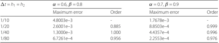
Table1shows the maximum absolute numerical error and temporal convergence or-ders for the ADI–implicit Euler method withTend= 1. From this table, we see that the

convergence order of the scheme isO(τ+h1+h2).

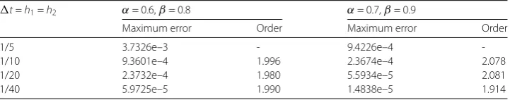
Table2shows the maximum error and temporal convergence orders for ADI–CN ex-trapolated solution withTend= 1. From this table, we see that the convergence order of

the scheme isO(τ2_+h2 1+h22).

Table 1 Maximum errors and temporal convergence orders for the ADI–implicit Euler method with Tend= 1

t=h1=h2 α= 0.6,β= 0.8 α= 0.7,β= 0.9

Maximum error Order Maximum error Order

1/10 4.8003e–3 - 1.7678e–3

-1/20 2.6001e–3 0.885 8.8503e–4 0.999

1/40 1.3000e–3 1.000 4.4357e–4 0.996

Table 2 Maximum errors and temporal convergence orders for ADI–CN extrapolated solution with T_end= 1

t=h1=h2 α= 0.6,β= 0.8 α= 0.7,β= 0.9

Maximum error Order Maximum error Order

1/5 3.7326e–3 - 9.4226e–4

-1/10 9.3601e–4 1.996 2.3674e–4 2.078

1/20 2.3732e–4 1.980 5.5934e–5 2.081

1/40 5.9725e–5 1.990 1.4838e–5 1.914

6 Conclusions

We use the shifted left Grünwald formula and the standard right Grünwald formula to approximate the left and right Riemann–Liouville fractional derivatives, respectively; we present an implicit Euler method and a CN method for the two-dimensional two-sided space-fractional diffusion equation. Two methods both combine with the ADI method to obtain unconditionally one-order accurate and two-order accurate finite difference meth-ods.

Acknowledgements

The authors would like to thank the referees for a careful reading and several constructive comments and making some useful corrections that have improved the presentation of the paper.

Funding

This work was supported by the National Natural Science Foundation of China (No. 11271141) and Chongqing Municipal Science and Technology Commission Fund Project (No. cstc2018jcyjAX0787).

Competing interests

The authors declare that they have no competing interests.

Authors’ contributions

All authors contributed equally to this work. All authors read and approved the final manuscript.

Author details

1_{School of Mathematics and Computation Science, Hunan University of Science and Technology, Xiangtan, China.} 2_{Department of Mathematics, South China Agricultural University, Guangzhou, China.}3_{School of Management,}

Guangdong University of Technology, Guangzhou, China.

Publisher’s Note

Springer Nature remains neutral with regard to jurisdictional claims in published maps and institutional affiliations.

Received: 8 December 2017 Accepted: 3 October 2018 References

1. Chen, S., Liu, F., Jiang, X., Turner, I., Anh, V.: A fast semi-implicit difference method for a nonlinear two-sided space-fractional diffusion equation with variable diffusivity coefficients. Appl. Math. Comput.257, 591–601 (2015) 2. Podlubny, I.: Fractional Differential Equations. Academic Press, New York (1999)

3. Meerschaert, M.M., Sikorskii, A.: Stochastic Models for Fractional Calculus. De Gruyter, Berlin (2012) 4. Liu, F., Meerschaert, M.M., Mcgough, R.J., Zhuang, P., Liu, Q.: Numerical methods for solving the multi-term

time-fractional wave-diffusion equation. Fract. Calc. Appl. Anal.16(1), 9–25 (2013)

5. Hao, Z.P., Sun, Z.Z., Cao, W.R.: A fourth-order approximation of fractional derivatives with its applications. J. Comput. Phys.281, 787–805 (2015)

6. Liu, F., Zhuang, P., Turner, I., Anh, V., Burrage, K.: A semi-alternating direction method for a 2-D fractional

FitzHugh-Nagumo monodomain model on an approximate irregular domain. J. Comput. Phys.293, 252–263 (2015) 7. Liu, T.H., Hou, M.Z.: A fast implicit finite difference method for fractional advection-dispersion equations with

fractional derivative boundary conditions. Adv. Math. Phys.2017, Article ID 8716752 (2017)

8. Zheng, M., Liu, F., Turner, I., Anh, V.: A novel high order space–time spectral method for the time fractional Fokker–Planck equation. SIAM J. Sci. Comput.37(2), 701–724 (2015)

9. Guo, B., Xu, Q., Zhu, A.: A second-order finite difference method for two-dimensional fractional percolation equations. Commun. Comput. Phys.19(3), 733–757 (2016)

10. Yin, X., Li, L., Fang, S.: Second-order accurate numerical approximations for the fractional percolation equations. J. Nonlinear Sci. Appl.10(8), 4122–4136 (2017)

12. Chen, H., Lv, W., Zhang, T.: A Kronecker product splitting preconditioner for two-dimensional space-fractional diffusion equations. J. Comput. Phys.360, 1–14 (2018)

13. Chen, M., Deng, W.: A second-order numerical method for two-dimensional two-sided space fractional convection diffusion equation. Appl. Math. Model.38(13), 3244–3259 (2014)

14. Liu, F., Chen, S., Turner, T., Burrage, K., Anh, V.: Numerical simulation for two-dimensional Riesz space fractional diffusion equations with a nonlinear reaction term. Cent. Eur. J. Phys.11(10), 1221–1232 (2013)

15. Zeng, F., Liu, F., Li, C., Burrage, K., Turner, I., Anh, V.: A Crank–Nicolson ADI spectral method for the two-dimensional Riesz space fractional nonlinear reaction-diffusion equation. SIAM J. Numer. Anal.52(6), 2599–2622 (2014) 16. Feng, L., Zhuang, P., Liu, F., Turner, I., Yang, Q.: Second-order approximation for the space fractional diffusion equation

with variable coefficient. Prog. Fract. Differ. Appl.1(1), 23–35 (2015)

17. Moroney, T., Yang, Q.: Efficient solution of two-sided nonlinear space-fractional diffusion equations using fast Poisson preconditioners. J. Comput. Phys.246(246), 304–317 (2013)

18. Chen, S., Liu, F., Jiang, X., Turner, I., Burrage, K.: Fast finite difference approximation for identifying parameters in a two-dimensional space-fractional nonlocal model with variable diffusivity coefficients. SIAM J. Numer. Anal.54(2), 606–624 (2016)

19. Feng, L.B., Zhuang, P., Liu, F., Turner, I.: Stability and convergence of a new finite volume method for a two-sided space-fractional diffusion equation. Appl. Math. Comput.257, 591–601 (2015)

20. Feng, L.B., Zhuang, P., Liu, F., Turner, I., Anh, V., Li, J.: A fast second-order accurate method for a two-sided space-fractional diffusion equation with variable coefficients. Comput. Math. Appl.73, 1155–1171 (2017) 21. Meerschaert, M.M., Tadjeran, C.: Finite difference approximations for fractional advection-dispersion flow equations.

J. Comput. Appl. Math.172, 65–77 (2004)

22. Tadjeran, C., Meerschaert, M.M., Scheffler, P.: A second order accurate numerical approximation for the fractional diffusion equation. J. Comput. Phys.213, 205–213 (2006)

23. Samko, S.G., Kilbas, A.A., Marichev, O.I.: Fractional Integrals and Derivatives: Theory and Applications. Gordon Breach, London (1993)

24. Meerschaert, M.M., Scheffler, H.P., Tadjeran, C.: Finite difference methods for two-dimensional fractional dispersion equation. J. Comput. Phys.211, 249–261 (2006)

25. Chen, S., Liu, F., Turner, I., Anh, V.: An implicit numerical method for the two-dimensional variable-order fractional percolation equation. Appl. Math. Comput.219, 4322–4331 (2013)