Dynamics of a diffusive Leslie–Gower predator–prey system with ratio dependent Holling III functional response

R E S E A R C H

Open Access

Dynamics of a diffusive Leslie–Gower

predator–prey system with ratio-dependent

Holling III functional response

Xiaoyuan Chang

_{and Jimin Zhang}

*_{Correspondence:} [email protected]

2_{School of Mathematical Sciences,}

Heilongjiang University, Harbin, P.R. China

3_{Heilongjiang Provincial Key}

Laboratory of the Theory and Computation of Complex Systems, Heilongjiang University, Harbin, P.R. China

Full list of author information is available at the end of the article

Abstract

This paper is devoted to investigating the dynamics of a diffusive Leslie–Gower predator–prey system with ratio-dependent Holling III functional response. We first establish the stability of positive constant equilibrium, and show the condition under which system undergoes a Hopf bifurcation with the explicit computational formulas for determining the bifurcating properties. Especially, when the positive constant equilibrium loses its stability, a supercritical Hopf bifurcation with spatial

homogeneous and stable bifurcating periodic solution occurs. Finally, we discuss the existence and nonexistence of nonconstant positive solutions with the help of Leray–Schauder degree theory and the implicit function theorem.

MSC: 92D25; 35K57

Keywords: Leslie–Gower predator–prey system; Hopf bifurcation; Nonconstant positive solutions; Equilibrium; Ratio-dependent Holling III functional response

1 Introduction

As one of the most common mutual relationships between two populations in nature, predator–prey relationship plays a significant role in ecology and mathematical biology. In mathematics, one way to model this relationship is by using differential equations with various types of predator’s functional responses, which is a key component of a predator– prey relationship. Leslie and Gower in [16,17] introduced a functional response, called Leslie–Gower functional response, to describe that reduction in predator population has a reciprocal relationship with per capita availability of its preferred food. A Leslie–Gower predator–prey system generally has the following form:

⎧ ⎪ ⎪ ⎨ ⎪ ⎪ ⎩ dx

dt =rx(1 – x

K) –yf(x),

dy

dt =y(1 – y px),

x(0) > 0,y(0) > 0,r,s,K,p> 0,

(1.1)

wherepis the conversion factor of the prey into the predator, and the termy/(px) is called the Leslie–Gower term representing the loss of the density of the predator due to rarity of the prey.

In recent years, there have been many theoretical results obtained for system (1.1) with different functional responsesf(x), such as Holling type I (f(x) =ax) [3,8,12,14], Holling type II (the so-called Holling–Tanner model,f(x) =mx/(b+x)) [2,8,9], Holling type III (f(x) =mx2_{/[(a+x)(b+x)]) [8,11], and Holling type IV (f(x) =mx/(b+x}2_{)) [19]. There}

is a recognition that spatial distribution patterns and dispersal mechanisms can cause the complexity and rich dynamical behavior of ecological modeling. The Leslie–Gower predator–prey system with diffusion has been investigated in a certain range [4–6,13, 22].

In characterizing predator’s functional response, ratio-dependent functional response is an important form. It is a predator-dependent functional response and has a better mod-eling for a predator–prey system [1,10,15,18,24,25,28,32]. Motivated by the existing studies and the above considerations, we replacef(x) byf(x/y) and consider spatial dis-tribution patterns and dispersal mechanisms in (1.1). Making a suitable nondimensional scaling, system (1.1) reduces to

⎧ ⎪ ⎪ ⎪ ⎪ ⎪ ⎨ ⎪ ⎪ ⎪ ⎪ ⎪ ⎩

∂u

∂t =d1u+u(1 –u) –

αu2_v

u2_+mv2, x∈Ω,t> 0,

∂v

∂t =d2v+βv(1 – v

u), x∈Ω,t> 0,

∂u

∂ν = ∂v

∂ν = 0, x∈∂Ω,t≥0,

u(0,x) =u0(x)≥≡0,v(0,x) =v0(x)≥≡0, x∈Ω,

(1.2)

whereu(x,t) andv(x,t) represent the densities of prey and predator at locationx∈ ¯Ωand timet≥0, respectively.Ω∈Rn_{(n∈N) is a bounded domain with smooth boundary∂Ω.}

d1andd2are diffusion coefficients, andα,m,βare positive constants. In [26], Shi and Li

introduced system (1.2) and established the stability of the positive equilibrium and uni-form persistence of the solution semiflows. Shi et al. in [27] considered the existence of the Turing–Hopf bifurcation where the Turing instability curve and the Hopf bifurcation curve intersect. Yang and Li in [30] obtained a sufficient condition for global asymptotic stability of the positive equilibrium by constructing recurrent sequences and using an it-erative method. Zhou in [33] established the existence and the bifurcating properties of Hopf bifurcation of system (1.2) by usingβas a bifurcating value.

The purpose of the present paper is to investigate dynamics of system (1.2), including the stability of the unique positive equilibrium, the existence and the bifurcating properties of Hopf bifurcation, the existence and nonexistence of nonconstant positive solutions. The main contributions have three aspects:

1. A larger parameter range of local stability of the unique positive constant equilibrium is established;

2. Using the predation rateαas the bifurcating value, we show that system (1.2) undergoes a Hopf bifurcation and derive the explicit computational formulas for determining the bifurcating properties. In particular, a supercritical Hopf bifurcation with spatial homogeneous and stable bifurcating periodic solutions occurs;

Our paper is organized as follows. In Sect.2, we establish the stability of the unique pos-itive constant equilibrium. In Sect.3, we discuss the condition under which system (1.2) undergoes a Hopf bifurcation and derive the explicit computational formulas for deter-mining the bifurcating properties. Especially, a supercritical Hopf bifurcation with spatial homogeneous and stable bifurcating periodic solutions occurs. Finally, we investigate the existence and nonexistence of nonconstant positive solutions by using a priori estimates, Leray–Schauder degree theory, and the implicit function theorem.

2 Stability of constant equilibria

In this section, we investigate the stability of constant equilibria of (1.2). From [26], we know that system (1.2) has a unique positive solution, denoted asE∗= (θ,θ) withθ= 1 – α/(1 +m), ifα< 1 +m. It is not difficult to see that system (1.2) has a semi-trivial constant solutionE1= (1, 0).

To discuss the stability of constant equilibria of system (1.2), we first make some no-tations. It is well known that the operator –inΩ with the homogeneous Neumann boundary condition has eigenvalues

μi∈Λ:={μi: 0 =μ0<μ1<· · ·<μi<· · ·,i∈N0} (2.1)

and the corresponding eigenfunctions areφij, whereN0:=N∪ {0}. LetS(μi) be the sub-space generated by the eigenfunctionsφijcorresponding toμi, m(μi) be the multiplic-ity of μi, and {φij}m(

μi)

j=1 be an orthonormal basis ofS(μi). DefineXij={cφij :c∈R2},

Xi=

m(μi)

j=1 Xij, and

X=(u,v)T∈C1(Ω¯) 2:∂νu=∂νv= 0 on∂Ω

satisfyingX=∞_i=0Xi.

The stability of the equilibria can be obtained by analyzing the distribution of the eigen-values of the characteristic equation corresponding to the linearized system of system (1.2). Then we have the following results.

Theorem 2.1 E1= (1, 0)is unstable.

Proof The linearized system of system (1.2) atE1can be written as

ϕt ψt

=D

ϕ ψ

+

–1 –α

0 β

ϕ ψ

, (2.2)

withD=diag(d1,d2). By using the fact above, the correspondingkth characteristic

equa-tion of (2.2) is

λ2––(d1+d2)μk+β– 1

λ+d1d2μ2k– (βd1–d2)μk–β

= 0. (2.3)

Whenk= 0, two roots of (2.3) are –1 andβ, which implies thatE1is unstable. Theorem 2.2 E∗is locally asymptotically stable if one of the following statements holds:

(B) m< 1andα≤(1+₂m)2; (C) m< 1,β<1–m

1+m,

(1+m)2

2 <α< (1 +β) (1+m)2

2 ,and

d1

d2 >d˜:=

1–m

β(1+m); (D) m< 1,β≥1–₁₊m_m, (1+₂m)2 <α< 1 +m,and d1

d2 >d˜.

Proof We now prove the local asymptotic stability ofE∗by analyzing the distribution of eigenvalues atE∗. The linearized system of system (1.2) atE∗is

ϕt ψt

=D

ϕ ψ

+

K1 K2

β –β

ϕ ψ

, (2.4)

and thekth characteristic equation of (2.4) is

λ2– TRk(α)λ+ DETk(α) = 0, (2.5)

where

K1=

2α

(1 +m)2– 1, K2=

α(m– 1)

(1 +m)2 (2.6)

and

TRk(α) = –(d1+d2)μk+K1–β,

DETk(α) =d1d2μ2k– (K1d2–βd1)μk+βθ. (2.7)

Note that if TRi(α) < 0 and DETj(α) > 0 for alli,j∈N0, thenE∗ is locally asymptotically

stable. It is clear that ifK1<β, then TR0(α) < 0 and TRk(α) < 0 for allk∈N. IfK1≤0, that

is,α≤(1 +m)2_{/2, then, obviously, TR}

k(α) < 0 and DETk(α) > 0 for allk∈N0. If 0 <K1<β,

that is, (1 +m)2/2 <α< (1 +β)(1 +m)2/2, then TR0(α) < 0 and TRj(α0) < 0 for allj∈N.

Note that

DETk(α) =d1d2μ2k–

2α (1 +m)2 – 1

d2–βd1

μk+βθ

>d1d2μ2k–

2(1 +m) (1 +m)2 – 1

d2–βd1

μk

=μk

d1d2μk–

1 –m

(1 +m)

d2–βd1

.

Then DETk(α) > 0 for allα< 1 +m, ifm< 1 andd1/d2> (1 –m)/(β(1 +m)) orm≥1. To

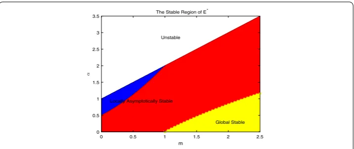
sum up above, we obtain the local stability ofE∗and complete the proof. Figure1shows the region of stability of equilibriumE∗in them–αplane.E∗is globally stable with them–αplane belonging to the yellow region, which is given as (ε0+θ)(1 +

m)2_ε2

0–α(1 –mε0)(1 +θ) > 0 withε0= 1 –α/(2 √

Figure 1The parameter ranges in them–αplane for the stability region ofE∗. Hered1= 3,d2= 0.5

3 Hopf bifurcation and its properites

In this section, we focus on the case that system (1.2) undergoes a Hopf bifurcation near

E∗ for the spatial domainΩ= (0,lπ) withl∈R+= (0, +∞). Then the eigenvalueμnis

n2/l2and the corresponding eigenfunctionφn(x) iscos(nx/l) for alln∈N0andx∈Ω. Our

results in this section can also be adapted to higher spatial domains. By cases (A) and (B) of Theorem2.2, the potential bifurcating value should satisfyα∈((1 +m)2_{/2, 1 +m) with}

m< 1. To study Hopf bifurcation nearE∗, we need to verify the condition under which the corresponding characteristic equations of the linearized operator of system (1.2) have a pair of simply pure imaginary roots, all other eigenvalues have non-zero real parts, and the transversality condition holds.

From [31], ifα∗is a Hopf bifurcation value, then there existsk∈N0such that

TRk

α∗= 0, DETk

α∗> 0, and

TRj

α∗= 0, DETj

α∗= 0, forj∈N0/{k},

(3.1)

and for the unique pair of complex eigenvaluesδ(α)±iω(α) near the imaginary axis,

δα∗= 0, (3.2)

where TRk(α) and DETk(α) are defined in (2.7).

Ifk= 0, then TR0(α) =K1–β, DET0(α) =βθ> 0. Let TR0(α) = 0, thenα=α0:= (1 +

β)(1 +m)2_{/2 withβ< (1 –m)/(1 +m), and TR}

j(α0) < 0, DETj(α0) > 0 ifd1/d2>d˜for allj∈N,

which implies that there exists a pair of simple pure imaginary roots of the characteristic equations of system (2.5) atE∗, and other eigenvalues has negative real parts.

We now consider α0 <α < 1 +m. It follows from TRk(α) = 0 that α =αk :=α0 +

(1 +m)2_(d

1+d2)k2/(2l2). In this case, for eachj∈N0/{k}, TRj(αk)= 0, DETj(αk) > 0 if

d1/d2>d˜. It is noted that there are only finite positive integers ksatisfying (3.1) since

αk∈(α0, 1 +m). Then the maximum positive integer, denoted asN1, is the integer part of

l(1 –m–β(1 +m))/((d1+d2)(1 +m)).

We next verify the transversality condition (3.2). Ifδ(α)±iω(α) are the roots of (2.5), then

δ(α) =TRk(α)

2 = –

(d1+d2)

2

k2

l2 +

α (1 +m)2–

1 +β

2 , ω(α) =

and

δα∗= 1 (1 +m)2 > 0,

whereα∗represents one of the bifurcating valuesαkwithk∈[0,N1].

Summarizing our analysis above, we obtain the following conclusion.

Theorem 3.1 Assume that m< 1andβ< (1 –m)/(1 +m).If d1/d2>d˜,then system(1.2)

undergoes a Hopf bifurcation near E∗atα=αk,where

αk=(1 +m)

2

2

1 +β+ (d1+d2)

k2

l2

, k∈[0,N1],

and N1is the integer part of l

(1 –m–β(1 +m))/((d1+d2)(1 +m)).Moreover,the spatial

homogeneous bifurcating periodic solutions bifurcate from α=α0, and the spatial

non-homogeneous bifurcating periodic solutions bifurcate fromα=αkwith k∈[1,N1].

We now establish the computational formulas for determining the properties of Hopf bi-furcation, including the bifurcating direction and stability of periodic solutions bifurcating fromE∗atα=αkwithk∈[0,N1], by using the normal form theory and the center

mani-fold argument presented in [7,31]. Fixk∈[0,N1], letα˜=αk,ω˜=ω(αk),θ˜= 1 –α˜/(1 +m), andλ=±iω(αk) =±iω˜ be the purely imaginary roots. By making the change of variables

u(x,t) –θ˜−→u(x,t) andv(x,t) –θ˜−→v(x,t), system (1.2) can be rewritten as an abstract form atα=α˜by

˙

U=L(α˜)U+F(α˜,U), (3.3)

whereU= (u,v)T_,

L(α˜) =

d1 0

0 d2

+

˜

K1 K˜2

β –β

=

d1 0

0 d2

+

2α˜

(1+m)2 – 1 ˜

α(m–1) (1+m)2

β –β

,

F(α˜,U) =

F1(α˜,U)

F2(α˜,U)

,

(3.4)

and

F1(α˜,U) =

A1

(1 +m)2_{((1 +m)θ}˜2_+u2_+mv2_{+ 2θ}˜_(u+mv)),

F2(α˜,U) =β(v+θ˜)

1 – v+θ˜

u+θ˜

–βu+βv–β(u–v)

2

u+θ˜ ,

A1= –(1 +m)3θ˜4+

2(1 +m)2– 2α˜u3– (1 +m)2u4+ 2m(1 +m)2–α˜uv2

–α˜(m– 1)mv3–mu2vα˜(3 +m) + (1 +m)2v– (1 +m)2θ˜3α˜– 1 + 4u

–m2α˜(1 –m) + (1 +m)2v2+u2α˜5 + 2m+m2+ (1 +m)2(2mv– 5) – (1 +m)θ˜26 + 7m+m2u2+m2α˜+ (1 +m)(–2 +v)v

+ 2uα˜(2 +m) + (1 +m)(2mv– 2 –m).

Define·,·to be the complex-valuedL2_{inner product on a Hilbert spaceX}

Cas

U1,U2= lπ

0

(u¯1u2+v¯1v2) dx, Ui= (ui,vi)T∈XC:=X+iXwithi= 1, 2.

Let

L∗(α˜) =

d1+K˜1 β ˜

K2 d2–β

.

Then the corresponding eigenfunctions ofL(α˜) andL∗(α˜) for eigenvaluesλ=±iω˜ are

q=q(x) = (1,bk)Tcos(kx/l), q∗=q∗(x) =

a∗_k,b∗_kTcos(kx/l), respectively, where

bk=

d1μk–K˜1 ˜

K2

+ ω_˜˜

K2

i, a∗_k= 1 2Γk

+K˜1–d1μk 2ωΓ˜ k

i,

b∗_k= K˜2 2ωΓ˜ k

i, Γk=

lπ

0

cos2

k lx

dx,

andqandq∗satisfyq∗,q= 1 andq∗,q¯= 0. LetX=XC⊕XSwith

XC={zq+z¯q¯:z∈C}, XS=U∈X:q∗,U= 0.

Thus, for any U= (u,v)T _{∈X, there existz∈Candw= (w}

1,w2)T∈XS such thatU=

zq+¯zq¯+w. Substituting it into system (3.3), we get

⎧ ⎨ ⎩ ˙

z=iω˜z+q∗,F0, ˙

w=L(α˜)w+H(z,z¯,w), (3.5)

where

H(z,¯z,w) =F0–

q∗,F0

q–q¯∗,F0

¯

q, (3.6)

and

F0=F(α˜,zq+z¯q¯+w) =

1 2QUU+

1

6CUUU+O

|U|4,

here,

and

Then comparing the coefficients of the same order ofzandz¯in (3.6) and (3.7), we have

+ω˜2+ 2K˜₂32ω˜2+ 5d2μk(K˜1–d1μk)

Then the coefficients in (3.9) determine the properties of the Hopf bifurcation as follows:

(i) μ∗₂determines the direction of the Hopf bifurcation: ifμ∗₂> (<)0, then the direction of the Hopf bifurcation is forward (backward), that is, the bifurcating periodic solutions exist withα> (<)α˜;

(iii) T2determines the period of the bifurcating periodic solutions: ifT2> (<)0, then the period increases (decreases).

In particular, whenk= 0, it follows from (3.9) that

c1(0) =

12m

(1 +m)2_{(β(1 +m) – (1 –m))}+i

β

6(1 +β)(m– 1)(1 +m)2_ω˜3

2(1 – 3m)2 +β27 +m(6 +m)(3 + 8m)+βm–26 +m(53 + 8m)– 7, (3.10) and

μ∗₂= 12m

(1 –m) –β(1 +m)> 0,

β₂∗= 24m

(1 +m)2_{(β(1 +m) – (1 –m))}< 0,

T2=

2(β2(m(–36 +m(–51 + 10m)) – 7) +β(7 +m(8 +m(–53 + 10m))) + 2(1 – 3m)2₎

3β(1 +β)(m– 1)(1 +m)2_{(β(1 +m) – 1 +m)}2 .

This means that whenα=α0, system (1.2) undergoes a supercritical Hopf bifurcation and

the bifurcating periodic solution is spatial homogeneous and orbital asymptotically stable.

Remark3.1 Compared with [33], here the reason for usingαas a bifurcating parameter is that we can give a more detailed analysis of Hopf bifurcation when the spatial homoge-neous bifurcating periodic solution comes out, including the accurate bifurcation direc-tion, the certain stability of bifurcating periodic soludirec-tion, and the computational formula of the tendency of the period.

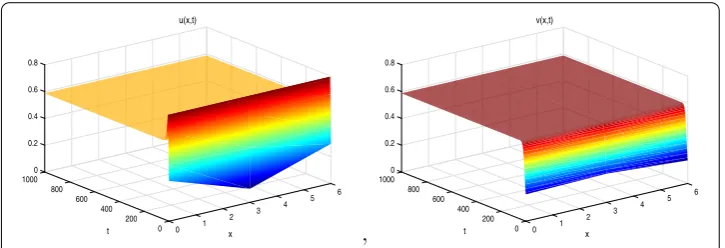
In order to illustrate our results, we do some numerical simulations for differentα. Let

d1= 3, d2= 0.5, l= 2, β= 0.1, m= 0.4 < 1,

u0= 0.2 + 0.1cosx, v0= 0.2 + 0.1sinx.

A straightforward calculation leads to the first bifurcating valueα0= 1.078. Whenα=

0.578 <α0, Fig.2shows that the solution of system (1.2) converges toE∗= (0.587, 0.587).

Whenα=α0, Fig.3shows that system (1.2) undergoes a Hopf bifurcation and the

peri-odic solution bifurcates fromE∗= (0.23, 0.23). In this case, using the formula of (3.10),

Figure 3System (1.2) undergoes a Hopf bifurcation nearE∗= (0.23, 0.23) withα= 1.078

c1(0) = –5.324 – 1.965iandT2= 3.244 > 0 imply that the period of the bifurcating periodic

solution increases.

4 Nonconstant positive solutions

In this section, we establish the nonexistence and existence of nonconstant positive solu-tion (u(x),v(x))∈[C2_(Ω)∩C1_(Ω¯_)]2_{of system (1.2), where (u(x),v(x)) satisfies}

⎧ ⎪ ⎪ ⎨ ⎪ ⎪ ⎩

d1u+u(1 –u) – αu

2_v

u2_+mv2 = 0, x∈Ω,

d2v+βv(1 –_uv) = 0, x∈Ω, ∂u

∂ν = ∂v

∂ν = 0, x∈∂Ω.

(4.1)

4.1 A priori estimates of nonnegative solutions

In this subsection, we derive a priori estimates of nonnegative solutions of system (4.1). We first introduce some known results.

Lemma 4.1(Maximum principle [21,22]) Assume that f ∈C(Ω)and cj∈C(Ω)with j= 1, 2, . . . ,n.

(i) Ifω∈C1_(Ω¯_)∩C2_{(Ω)satisfies} ⎧

⎨ ⎩

ω+n_j=1cj(x)ωxj+f(x)≥0, x∈Ω,

∂νω≤0, x∈∂Ω

andω(x0) =maxx∈ ¯Ωω(x),thenf(x0)≥0. (ii) Ifω∈C1_(Ω¯_)∩C2_{(Ω)satisfies}

⎧ ⎨ ⎩

ω+n_j=1cj(x)ωxj+f(x)≤0, x∈Ω,

∂νω≥0, x∈∂Ω

andω(x0) =minx∈ ¯Ωω(x),thenf(x0)≤0.

Lemma 4.2(Harnack inequality [20,22]) If u∈C2_(Ω)∩C1_(Ω¯_{)is a positive solution of} ⎧

⎨ ⎩

u(x) +b(x)u(x) = 0, x∈Ω,

where b∈C(Ω)∩L∞(Ω),then there exists a positive constant L which depends only on M,

satisfyingb∞≤M,such that

max x∈ ¯Ω

u(x)≤Lmin x∈ ¯Ωu(x).

We now establish a priori estimates of nonnegative solutions of system (4.1).

Theorem 4.1 If(u(x),v(x))is a positive solution of system(4.1),then

0 <min x∈ ¯Ω

u(x)≤min x∈ ¯Ω

v(x)≤max x∈ ¯Ω

v(x)≤max x∈ ¯Ω

u(x)≤1.

Proof Assume that (u(x),v(x)) is a positive solution of system (4.1). From the first equation of system (4.1), we have

d1u+u(1 –u) =

αu2_v

u2_+mv2≥0.

Let u(x0) =maxx∈ ¯Ωu(x). From Lemma 4.1, we have u(x0)(1 – u(x0))≥ 0, that is,

max_{x∈ ¯Ω}u(x)≤1.

Letv(x1) =maxx∈ ¯Ωv(x). Then we have

0≤βv(x1)

1 – v(x1)

u(x1)

≤βv(x1)

1 –v(x1)

u(x0)

,

that is,max_{x∈ ¯Ω}v(x)≤max_{x∈ ¯Ω}u(x).

Letv(x2) =minx∈ ¯Ωv(x). It follows from Lemma4.1that

βv(x2)

1 –v(x2)

u(x2)

≤0,

that is,min_{x∈ ¯Ω}v(x)≥u(x2)≥minx∈ ¯Ωu(x).

Theorem 4.2 Assume thatd is a positive constant¯ .If d1>d¯,then there is a positive

con-stant L such that each positive solution(u(x),v(x))of system(4.1)satisfies

0 <max x∈ ¯Ω

u(x)≤Lmin x∈ ¯Ω

u(x).

Proof Let

b(x) =u(x)

d1

1 –u(x) – αu(x)v(x)

u2_{(x) +mv}2_(x)

.

Then the first equation of system (4.1) can be written as

u(x) +b(x)u(x) = 0. (4.2)

From Theorem4.1, we haveb(x)∈C(Ω)∩L∞(Ω). It follows from Lemma4.2that the

From Theorems4.1and4.2, we conclude that there exists a positive constantκ such that

min x∈ ¯Ωu(x)≥

κ, min

x∈ ¯Ωv(x)≥

κ (4.3)

for anyd1≥ ¯dand any positive solution (u(x),v(x)) of system (4.1). By using the standard

Schauder theory for elliptic equations, we also conclude that there exists a positive con-stantκ¯such that

u2+γ ≤ ¯κ, v2+γ ≤ ¯κ (4.4)

for alld1,d2≥ ˆdand each positive solution (u,v)∈C2+γ(Ω¯)×C2+γ(Ω¯) of system (4.1),

wheredˆis a positive constant andγ ∈(0, 1).

4.2 Nonexistence of nonconstant positive solutions

In this subsection, we explore the nonexistence of nonconstant positive solutions of sys-tem (4.1) for different diffusion coefficientsd1,d2.

We first show that if diffusion coefficients of predator and prey are both sufficiently large, then system (4.1) has no nonconstant positive solutions. Letu¯=|Ω|–1

Ωu(x) dxandv¯= |Ω|–1_Ωv(x) dxfor any positive solution (u,v) of system (4.1). It is clear that_Ω(u–u¯) dx=

Ω(v–v¯) dx= 0. Multiplying the first equation of system (4.1) byu–u¯ and the second

equation of system (4.1) byv–v¯, then integrating onΩ, respectively, we have

d1

Ω

_∇(u–u¯)2dx=

Ω

(u–u¯)u(1 –u) dx–

Ω

(u–u¯) αu

2_v

u2_+mv2dx

=L1(u,u¯) +L2(u,u¯,v), (4.5)

d2

Ω

_∇(v–v¯)2dx=β

Ω

(v–v¯)

v

1 – v

u

–¯v

1 – ¯v

¯

u

dx

=β

Ω

(v–v¯)2dx+L3(u,v,¯v), (4.6)

and the following.

Theorem 4.3 Let d0be a positive constant.Then system(4.1)has no nonconstant positive

solutions for any d1,d2>d0.

Proof Assume that (u,v) is a positive solution of system (4.1). From Theorem4.1and (4.3), we haveκ≤u,v≤1 andκ≤ ¯u,v¯≤1 for anyx∈ ¯Ω. Then

L1(u,u¯) =

Ω

(u–u¯)u(1 –u) –u¯(1 –u¯) dx

=

Ω

(u–u¯)2(1 –u–u¯) dx

≤ Ω

L2(u,u¯,v) = –α

Combining (4.7) and (4.8) and applying the Poincaré inequality, we have

d1

We now prove that if the ability of the predators to hunt is strong and the predators move slow or the preys move fast, then system (4.1) has no nonconstant positive solutions.

Lemma 4.3 If(u,v)is a nonconstant positive solution of system(4.1),then

0 <η¯:=min x∈ ¯Ω

v(x)

Proof If the conclusion is not true, thenv(x)≥≡u(x) for anyx∈ ¯Ω. Integrating the second

which is a contradiction.

Theorem 4.4 Ifα≥1 +m and d2/d1≤β,then system(4.1)has no nonconstant positive

We next show that if the ability of the predators to hunt is weak and the preys move fast, then system (4.1) has no nonconstant positive solution. For 0 <γ< 1, we let

Y1=

u∈Cγ(Ω¯) :

Ω

udx= 0

,

Y2=

u∈C2+γ_(Ω¯_{) :∂}

νu= 0 on∂Ω

, Y3=Y1∩Y2,

u=τ+ωwithτ∈Randω∈Y3. Letξ=d–11 and

h1(ξ,τ,ω,v) =

1

|Ω|

Ω

(τ+ω)(1 –τ–ω) – α(τ+ω)

2_v

(τ+ω)2_+mv2

dx,

h2(ξ,τ,ω,v) =ω+ξ(τ+ω)(1 –τ–ω) –

ξ α(τ+ω)2_v

(τ+ω)2_+mv2 –ξf1(ξ,τ,ω,v),

h3(ξ,τ,ω,v) =d2v+βv

1 – v

τ+ω

,

H(ξ,τ,ω,v) = (h1,h2,h3)T(ξ,τ,ω,v).

It is clear thatH:R2×Y3×Y2→R×Y1×Cγ(Ω¯) and (u,v) is a solution of system (4.1)

if and only ifH(ξ,τ,ω,v) = 0. It follows that

Φ(τ,ω,v) :=H(τ,ω,v)(0,θ, 0,θ) = ⎛ ⎜ ⎝

|Ω|–1_Ω(K1τ+K1ω+K2v) dx ω

d2v–βv+βτ+βω ⎞ ⎟ ⎠,

whereθ= 1 –α/(1 +m),K1andK2are defined in (2.6). A straightforward calculation yields

the following.

Lemma 4.4 Φis an isomorphism.

Proof To obtain the conclusion, we only need to prove that

|Ω|–1

Ω

(K1τ+K1ω+K2v) dx=τ¯, (4.10)

ω=ω¯, x∈Ω, ∂νω|∂Ω= 0,

Ω

ωdx= 0, (4.11)

⎧ ⎨ ⎩

d2v–βv=v¯–β(τ+ω), x∈Ω,

∂νv= 0, x∈∂Ω

(4.12)

has a unique solution for any given (τ¯,ω¯,v¯)∈R×Y1×Cγ(Ω¯).

It is easy to see that system (4.11) has a unique solutionω∈Y3sinceω¯∈Y1. From (4.10)

and (4.11), we have

Ω

Integrating the first equation of system (4.12) overΩ, we obtain

τ=

Ω ¯

vdx+τ β¯ |Ω||Ω|β(K1+K2) –1

. (4.13)

Then system (4.12) has a unique solutionv, andvsatisfies

β

Ω

vdx=βτ|Ω|–

Ω ¯

vdx. (4.14)

This means thatΦis an isomorphism.

Letdi₁∈(0, +∞) and (ui_,vi_{) be positive solutions of system (4.1) withd}

1=di1. By using a

method similar to that mentioned in [23], we have the following lemma.

Lemma 4.5 Assume thatα< 1 +m and(ui_,vi_{)→(u˜,v˜)uniformly on Ω}¯ _{as d}i

1→ ˜d1∈

[0, +∞].Ifu and˜ ˜v are positive constants,then(u˜,v˜) = (θ,θ).

Theorem 4.5 Assume thatα< 1 +m andd˜11is a fixed constant.Then system(4.1)has

no nonconstant positive solution for any d1>d˜1.

Proof We claim that system (4.1) has only a positive solution (θ,θ) in a small neighborhood of (θ,θ). In fact, it follows from Lemma4.4thatΦ–1exists and is a bounded linear operator. By using the implicit function theorem, we conclude that there exists a constantε> 0 such that, for all 0 <ξ<ε,H(ξ,τ,ω,v) = 0 has a unique positive solution (θ, 0,θ) in the small neighborhoodBε(θ, 0,θ). This implies that whend1> 1/ε, system (4.1) has only a positive

solution (θ,θ) inBε(θ,θ).

Assume that (ui_,vi_{) is the nonconstant positive solution of system (4.1) withd}

1=d1i ∈

(0, +∞) anddi

1→+∞. It follows from (4.4) that (ui,vi)→(uˆ,vˆ) in [C2(Ω¯)]2asdi1→+∞.

From Theorem4.1and (4.3), we conclude that (uˆ,vˆ) is bounded anduˆ> 0 satisfies

–ˆu= 0, x∈Ω, ∂νuˆ= 0, x∈∂Ω.

This means thatuˆis a positive constant. Substituting it into the second equation of system (4.1), we get

v+βv(1 –v/uˆ) = 0, x∈Ω, ∂νv= 0, x∈∂Ω,

which implies thatv=uˆ. It follows from Lemma4.5and (ui_,vi_{)→(uˆ,vˆ) that (uˆ,vˆ)≡(θ,θ)} and there existsi0such that (ui,vi) = (θ,θ) for anyi≥i0and eachdi1> 1/ε. This is a

con-tradiction to that (ui_,vi_{) is a nonconstant positive solution of system (4.1).}

4.3 Existence of nonconstant positive solutions

exists a unique positive constant solutionE∗= (θ,θ) ifα< 1 +m. Let

W(U) :=

u(1 –u) –_u2α₊u_mv2v2

βv(1 –_uv)

(4.15)

withU= (u,v)T_{∈Xand (I–)}–1_{be the inverse ofI–. Then system (4.1) can reduce to}

G(d1,d2,U) :=U– (I–)–1

D–1W(U) +U= 0, (4.16)

whereI–satisfies the homogeneous Neumann boundary condition. Frechét derivative of system (4.16) with respect toUat (θ,θ) is

GU(d1,d2,θ,θ) =I– (I–)–1

D–1WU(θ,θ) +I

= 0.

Obviously,ζis an eigenvalue ofGU(d1,d2,θ,θ) onXiwithi∈N0if and only ifζ(1 +μi) is an eigenvalue of the matrix

Li:=μiI–D–1WU(θ,θ) =

μi–K1/d1 –K2/d1

–β/d2 μi+β/d2

, (4.17)

whereK1andK2are defined in (2.6). Then

detLi= 1

d1d2

d1d2μ2i– (d2K1–βd1)μi+βθ

= 1

d1d2

S(d1,d2,μi),

where

S(d1,d2,μ) :=d1d2μ2– (d2K1–βd1)μ+βθ. (4.18)

In order to obtain the existence of nonconstant positive solutions of system (4.1), we need the following two lemmas.

Lemma 4.6 If m< 1,α∈((1 +m)2_{/2, 1 +m)and d}

1/d2<d–,then S(d1,d2,μ) = 0has two

positive roots

μ±(d1,d2) =

d2K1–βd1± √

S 2d1d2

, (4.19)

where

S= (d2K1–βd1)2– 4d1d2βθ, and d–=

2θ+K1– 2

θ(θ+K1)

/β.

Proof It is not difficult to show thatS(d1,d2,μ) = 0 has two positive roots if and only if

S≥0 and

l(d1,d2) =

K1d2–βd1

2d1d2

= 1

2d1d2

d2

2α (1 +m)2– 1

–d1β

A direct calculation gives

S=β2d21+ 2β

2αm

(1 +m)2 – 1

d1d2+K12d22

=d2₂

β2

d1

d2 2

+ 2β

2αm

(1 +m)2 – 1

d1

d2

+K₁2

.

Note that ifα> (1 +m)2/2 andd1/d2<K1/β, thenl(d1,d2) > 0. Combining withα< 1 +m

implies thatm< 1. This means that 2αm/(1 +m)2_{– 1 < 0. Let}

r(d) =β2d2+ 2β

2αm

(1 +m)2 – 1

d+K₁2.

The discriminant of the roots ofr(d) = 0 isr= 16β2θ(θ+K1) > 0. Hence,r(d) = 0 has

two positive roots

d±=1

β

2θ+K1±2

θ(θ+K1)

. (4.20)

Whend<d–ord>d+, we getr(d) > 0. On the other hand,r(K1/β) = –4K1θ < 0. That is,

ifd1/d2<d–, thenS> 0 andl(d1,d2) > 0. This shows that (4.19) holds.

For a fixedd1> 0, ifd2is sufficiently large, thend1/d2<d–holds. Let

R(d1,d2) =

μ≥0 :μ–(d1,d2) <μ<μ+(d1,d2)

.

From (4.19), we have

lim d2→+∞

μ–(d1,d2) = 0, lim

d2→+∞

μ+(d1,d2) =K1/d1> 0. (4.21)

Lemma 4.7 ([23, 29]) If S(d1,d2,μi)= 0for all μi∈Λ,then index(G(d1,d2,·), (θ,θ)) =

(–1)σ_,whereσ=

μi∈R(d1,d2)∩Λm(μi)whenR(d1,d2)∩Λ=φandσ= 0whenR(d1,d2)∩

Λ=φ.In particular,if S(d1,d2,μ) > 0for allμ≥0,thenσ= 0.

Theorem 4.6 Assume that d1 andβ are fixed positive constants and m< 1, α∈((1 +

m)2_{/2, 1 +m),K}

1/d1∈(μk,μk+1)for some k∈N.If k

i=1m(μi)is odd,then there exists a

positive constantdˆ2such that,for any d2≥ ˆd2, (4.1)has at least one nonconstant positive

solution.

Proof From (4.21) andK1/d1∈(μk,μk+1), there existsd¯21 such that, for anyd2>d¯2,

0 <μ–(d1,d2) <μ1<· · ·<μk<μ+(d1,d2) <μk+1. (4.22)

It follows from Theorem4.3that system (4.1) has no nonconstant positive solutions for anyd1,d2>d0. We choosedˆ1>d0anddˆ2>max{¯d2,d0}such thatK1/dˆ1<μ1and

0 <μ–(dˆ1,dˆ2) <μ+(dˆ1,dˆ2) <μ1. (4.23)

If the conclusion of Theorem4.6is not true, then there is somed2such that system (4.1)

t)dˆ1,td2+ (1 –t)dˆ2) and consider the following system: ⎧

⎨ ⎩

–DtU=W(U), x∈Ω,

∂νU= 0, x∈∂Ω,

(4.24)

whereW(U) is defined in (4.15). It is clear that (4.24) is equivalent to

Ψ(U,t) =U– (I–)–1D–1_t W(U) +U= 0, U∈X.

Note thatΨ(U, 1) =G(d1,d2,U),Ψ(U, 0) =G(dˆ1,dˆ2,U) and

GU(d1,d2,θ,θ) =I– (I–)–1

diag(d1,d2)–1WU(θ,θ) +I

= 0,

GU(dˆ1,dˆ2,θ,θ) =I– (I–)–1

diag(dˆ1,dˆ2)–1WU(θ,θ) +I

= 0.

It follows from Theorems4.5and4.3thatΨ(U, 1) = 0 andΨ(U, 0) = 0 have no noncon-stant positive solutions.

By using (4.22) and (4.23), we have

R(d1,d2)∩Λ={μ1,μ2, . . . ,μk}, R(dˆ1,dˆ2)∩Λ=φ,

which implies that

indexΨ(·, 1), (θ,θ)= (–1)ki=1m(μi)_{= –1, indexΨ(}·_{, 0), (θ,θ)= (–1)}0_{= 1.}

From Theorem4.1and (4.3), we haveκ/2 <u,v< 2 for any solution (u,v) of system (4.1) onΩ¯. Let

Θ=(u,v)T∈X:κ/2 <u,v< 2,x∈ ¯Ω.

ThenΨ(U,t)= 0 on∂Θfor allt∈[0, 1]. It follows from the homotopy invariance of Leray– Schauder degree that

degΨ(·, 0),Θ, 0=degΨ(·, 1),Θ, 0. (4.25)

Note thatΨ(U, 0) = 0 andΨ(U, 1) = 0 have only the constant solution (θ,θ) inΘ and hence,

degΨ(·, 0),Θ, 0=indexΨ(·, 0), (θ,θ)= 1,

degΨ(·, 1),Θ, 0=indexΨ(·, 1), (θ,θ)= –1,

which is a contradiction to (4.25). The proof is complete.

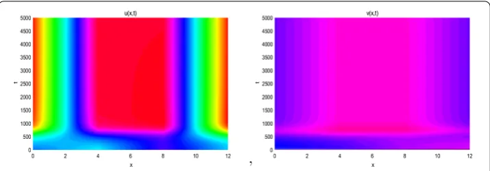
From Theorem4.6, ifd2/d1 is large enough andm< 1, then Fig.4shows that system

Figure 4The nonconstant positive solution of system (1.2). Hered1= 0.005,d2= 20,α= 1,m= 0.4,β= 0.1

Acknowledgements Not applicable.

Funding

This research is partially supported by Merit-based Funding for Returned Overseas Students of Heilongjiang Province, Heilongjiang Postdoctoral Funds for Scientific Research Initiation (Q17148).

Competing interests

The authors declare that they have no competing interests.

Authors’ contributions

All authors contributed equally to the manuscript and typed, read, and approved the final manuscript.

Author details

1_{School of Applied Sciences, Harbin University of Science and Technology, Harbin, P.R. China.}2_{School of Mathematical}

Sciences, Heilongjiang University, Harbin, P.R. China.3_{Heilongjiang Provincial Key Laboratory of the Theory and}

Computation of Complex Systems, Heilongjiang University, Harbin, P.R. China.

Publisher’s Note

Springer Nature remains neutral with regard to jurisdictional claims in published maps and institutional affiliations.

Received: 2 November 2018 Accepted: 12 February 2019

References

1. Abrams, P.A., Ginzburg, L.R.: The nature of predation: prey dependent, ratio dependent or neither? Trends Ecol. Evol.

15, 337–341 (2000)

2. Barza, P.A.: The bifurcation structure of the Holling–Tanner model for predator–prey interactions using two-timing. SIAM J. Appl. Math.63, 889–904 (2003)

3. Chen, F., Chen, L., Xie, X.: On a Leslie–Gower predator–prey model incorporating a prey refuge. Nonlinear Anal., Real World Appl.10, 2905–2908 (2009)

4. Chen, S., Shi, J.: Global stability in a diffusive Holling–Tanner predator–prey model. Appl. Math. Lett.25, 614–618 (2012)

5. Chen, S., Shi, J., Wei, J.: Global stability and Hopf bifurcation in a delayed diffusive Leslie–Gower predator–prey system. Int. J. Bifurc. Chaos22, 1250061 (2012)

6. Du, Y., Hsu, S.B.: A diffusive predator–prey model in heterogeneous environment. J. Differ. Equ.203, 331–364 (2004) 7. Hassard, B.D., Kazarinoff, N.D., Wan, Y.H.: Theory and Applications of Hopf Bifurcation. Cambridge University Press,

Cambridge (1981)

8. Hsu, S.B., Huang, T.W.: Global stability for a class of predator–prey systems. SIAM J. Appl. Math.55, 763–783 (1995) 9. Hsu, S.B., Huang, T.W.: Hopf bifurcation analysis for a predator–prey system of Holling and Leslie type. Taiwan. J. Math.

3, 35–53 (1999)

10. Hsu, S.B., Huang, T.W., Kuang, Y.: Global analysis of the Michaelis–Menten type ratio-dependent predator–prey system. J. Math. Biol.42, 489–506 (2001)

11. Huang, J., Ruan, S., Song, J.: Bifurcations in a predator–prey system of Leslie type with generalized Holling type III functional response. J. Differ. Equ.257, 1721–1752 (2014)

12. Huo, H., Li, W.: Stable periodic solution of the discrete periodic Leslie–Gower predator–prey model. Math. Comput. Model.40, 261–269 (2004)

13. Jiang, J., Song, Y.: Delay-induced Bogdanov–Takens bifurcation in a Leslie–Gower predator–prey model with nonmonotonic functional response. Commun. Nonlinear Sci. Numer. Simul.19, 2454–2465 (2014)

14. Korobeinikov, A.: A Lyapunov function for Leslie–Gower predator–prey models. Appl. Math. Lett.14, 697–699 (2001) 15. Kuang, Y., Beretta, E.: Global qualitative analysis of a ratio-dependent predator–prey system. J. Math. Biol.36, 389–406

(1998)

17. Leslie, P.H., Gower, J.C.: The properties of a stochastic model for the predator–prey type of interaction between two species. Biometrika47, 219–234 (1960)

18. Li, Y., Wang, M.: Stationary pattern of a diffusive prey–predator model with trophic intersections of three levels. Nonlinear Anal., Real World Appl.14, 1806–1816 (2013)

19. Li, Y., Xiao, D.: Bifurcations of a predator–prey system of Holling and Leslie types. Chaos Solitons Fractals34, 606–620 (2007)

20. Lin, C., Ni, W., Takagi, I.: Large amplitude stationary solutions to a chemotaxis system. J. Differ. Equ.72, 1–27 (1988) 21. Lou, Y., Ni, W.: Diffusion vs cross-diffusion: an elliptic approach. J. Differ. Equ.154, 157–190 (1999)

22. Ni, W., Wang, M.: Dynamics and patterns of a diffusive Leslie–Gower prey–predator model with strong Allee effect in prey. J. Differ. Equ.261, 4244–4274 (2016)

23. Pang, P.Y.H., Wang, M.: Non-constant positive steady states of a predator–prey system with non-monotonic functional response and diffusion. Proc. Lond. Math. Soc.88, 135–157 (2004)

24. Pang, P.Y.H., Wang, M.: Strategy and stationary pattern in a three-species predator–prey model. J. Differ. Equ.200, 245–273 (2004)

25. Peng, R., Wang, M., Yang, G.: Stationary patterns of the Holling–Tanner prey–predator model with diffusion and cross-diffusion. Appl. Math. Comput.196, 570–577 (2008)

26. Shi, H., Li, Y.: Global asymptotic stability of a diffusive predator–prey model with ratio-dependent functional response. Appl. Math. Comput.250, 71–77 (2015)

27. Shi, H., Ruan, S., Su, Y., Zhang, J.: Spatiotemporal dynamics of a diffusive Leslie–Gower predator–prey model with ratio-dependent functional response. Int. J. Bifurc. Chaos25, 1530014 (2015)

28. Wang, M.: Stationary patterns for a prey–predator model with prey-dependent and ratio-dependent functional responses and diffusion. Physica D196, 172–192 (2004)

29. Wang, M.: Nonlinear Elliptic Equations. Academic Press, San Diego (2010) in Chinese

30. Yang, W., Li, X.: Global asymptotical stability for a diffusive predator–prey model with ratio-dependent Holling type III functional response. Differ. Equ. Dyn. Syst. 1–9 (2017)

31. Yi, F., Wei, J., Shi, J.: Bifurcation and spatiotemporal patterns in a homogenous diffusive predator–prey system. J. Differ. Equ.246, 1944–1977 (2009)

32. Zhao, J., Zhang, H., Yang, J.: Stationary patterns of a ratio-dependent prey–predator model with cross-diffusion. Acta Math. Appl. Sin. Engl. Ser.33, 497–504 (2017)