R E S E A R C H
Open Access
Multigrid method based on
transformation-free high-order scheme for
solving 2D Helmholtz equation on
nonuniform grids
Fazal Ghaffar
1, Noor Badshah
2, Saeed Islam
1and Muhammad Altaf Khan
1**Correspondence: [email protected] 1Department of Mathematics, Abdul Wali Khan University, Mardan, Pakistan
Full list of author information is available at the end of the article
Abstract
High-order compact difference schemes can achieve higher-order accuracy on uniform grids. However, in some cases these may not achieve the desired accuracy. Therefore, we propose a multigrid method based on high-order compact difference scheme on nonuniform grids. We will use interpolation and restriction operators developed by Ge and Cao (J. Comput. Phys. 230:4051-4070, 2011). The suggested scheme has up to fourth-order accuracy. Lastly, some numerical experiments are given to show the accuracy and performance of the proposed scheme.
MSC: 65Nxx; 65Mxx
Keywords: Helmholtz equation; compact iterative schemes; multigrid method; nonuniform grids
1 Introduction
Two- and three-dimensional elliptic partial differential equations (PDEs) play a pivotal role in different fields of science and technology. High-order compact schemes (HOC) are used for the solution of the Helmholtz equation and other elliptic PDEs [, ]. Consider the two-dimensional (D) Helmholtz equation
uxx+uyy+ku=f(x,y), (x,y)∈, ()
whereis a rectangular domain andkis a wave number. The forcing functionf(x,y) and the solutionu(x,y) have the required continuous differentiability up to a specific order. The equation has many real-world applications like elasticity, electromagnetic waves, acoustic wave scattering, weather and climate prediction, water wave propagation, noise reduction in silencers, and radar scattering. In this paper, we use a finite-difference approximation on nonuniform grids in discrete domain to obtain a scheme up to fourth-order accuracy. We also considered the Helmholtz equation with constant value ofk.
Equation () has been solved by different techniques such as finite-difference method (FDM) [], fast-Fourier-transform-based (FFT) methods [], finite-element method (FEM) [], the spectral-element method [], compact finite-difference method [], and
multigrid methods []. The multigrid method based on HOC schemes is among the most efficient iterative techniques for solving PDEs [, ].
In FDM the number of mesh points will be enlarged to increase the accuracy; however, it will also increase the computational time. The Helmholtz equation is solved by FEM and spectral-element method, but the limitations of these methods are of high computa-tional cost []. Many iterative techniques for the Helmholtz equation suffer due to their slow convergence. The investigation on fast iterative methods to efficiently solve the large algebraic systems arising from high-order difference schemes for PDEs is more attractive. Multigrid methods together with the HOC schemes on uniform mesh sizes are developed in [–]. In most cases where sudden changes occur in a flow, the step sizes have to be rectified over the entire domain. Under these situations, where points are concentrated in the regions of sharp variation, local mesh refinement procedures [, , , –] are nec-essary, thus dramatically reducing the computational time and computer storage. Ge and Cao [, ] developed a multigrid method with HOC scheme on nonuniform grids for solv-ing D convection diffusion equation and D Poisson equation. This paper is based on ap-proach that an interpolation operator and a projection operator that are suited for a HOC scheme using nonuniform mesh are represented by a transformation-free HOC scheme on nonuniform grids. The main focus in this paper is to develop a multigrid method based on a HOC scheme on nonuniform grids for solving of the D Helmholtz equation. To the best of our knowledge, the D Helmholtz equation is not solved by a multigrid method based on a HOC scheme on nonuniform grids.
2 HOC scheme on nonuniform grids
Consider a square domain (x,y)∈[a,a]×[b,b]. Discretization is performed on
two-dimensional nonuniform gird points. The interval [a,a] is divided into subintervals
a=x,x,x, . . . ,xNx=a, b=y,y,y, . . . ,yNy=b.
In thex-direction, considerhx=aNx–a, and the forward and backward step sizes are given by
hfx=xi+–xi=θfxhx, hbx=xi–xi–=θbxhx, ≤i<Nx– . Similarly in they-direction,hy=bNy–b,
hfy=yj+–yj=θfyhy, hby=yj–yj–=θbyhy, ≤j<Ny– .
Furthermore,αx=θfxθbx,βx=θfx+θbx, andγx=θfx–θbx. Ifθfx=θbx= (hfx=hbx,hfy=
hby), then the grids turn to be uniform. The approximate values of a functionu(x,y) at interior grid points (xi,yj) are represented byu, and the estimated values of other eight
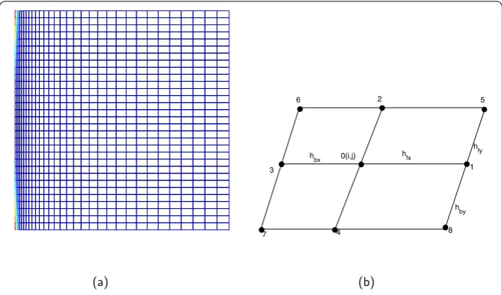
neighboring points are determined byui,i= , , , . . . , , as in Figure .
The Taylor series expansion is performed for appropriate description of a sufficiently smooth functionu(x,y) in the given domain at points and , which are
u=u+θfxhx∂xu+
θfxhx
∂
xu+
θfxhx
∂
xu
+θ
fxhx
∂
xu+
θfxh
x
∂
xu+O
Figure 1 Nonuniform grids inxy-plane. (a)Nonuniform grids distribution inxy-plane.(b)Stencil of
Multiplying equation () byθbxand () byθfx, then adding and solving for the second-order derivative, which gives
x-direction is defined as
δxu=
αxβxhx
(θbxu–βxu+θfxu); ()
ifθfx=θbx= , then equation () reduces to uniform grids of the central difference operator. Hence, the second-order derivative for thex-direction is
∂xu=δxu–
and the approximation of the second-order derivative for the variableycan be find ac-cordingly. Therefore, the central difference (CD) scheme for the Helmholtz equation can be discretized as
whereτis the truncation error and is defined as
Ifτis dropped off from equation (), then the CD scheme for nonuniform grids becomes
δxu+δyu+k(u) =f. ()
According to the definition ofδ
x,δy, the CD scheme can be written as
In equation (), only five grid points are involved. From the definition ofτwe can see
that whenhfx=hbxandhfy=hby, then equation () is of second-order accuracy. In order to improve the accuracy, we consider
Applying the central difference scheme to equation (), we have
Similarly, equation () will be
H
Through central difference schemes, the first- and second-order derivatives in equations (), () can be approximated. Now combining equations () and () with equations () and (), the nine-point HOC scheme on nonuniform mesh points for two-dimensional Helmholtz equation () can be written as
The coefficients of the LHS in equation () are given as
A=
Lθfx
αxβxβyhxhy
– Hθby
αyβxβyhxhy
+(H+L)θbyθfx
αxαyβxβyhxhy ,
A=
–Lθbx
αxβxβyhxhy
+ Hθfy
αyβxβyhxhy
+(H+L)θfyθbx
αxαyβxβyhxhy ,
A=
–Hθfy
αyβxβyhxhy
– Lθfx
αxβxβyhxhy
+(H+L)θfxθfy
αxαyβxβyhxhy .
It is easier to know that this scheme has third to fourth order of accuracy from expansion ofτ.
3 Multigrid method
The multigrid method is one of the most efficient and fastest methods for solving PDEs. In the multigrid method, the rate of convergence is independent of the mesh size. This method is more effective for solving large-scale sparse linear systems obtained from the discretization of elliptic PDEs [, , –]. The main principle of the multigrid method is to smoothen the error on coarse grid level using basic iterative methods such as Jacobi or Gauss-Seidel method,etc.The multigrid method consists of three important components that are relaxation, restriction, and interpolation operators. These are applied as ‘a single iteration of a multigrid cycle comprised of manipulating the error by the application of relaxation method, fixing the residuals on the coarse grid level, solving the error equation on the coarse grid and adjusting the correction of coarse grid up to the fine grid level’.
Some specific methods have been applied for the solution of the D and D Helmholtz equations with HOC schemes on uniform grids [–, , , , ]. A full weighting restric-tion operator and the standard bilinear interpolarestric-tion operator are used as the inter-grid transfer operators. But in the case of nonuniform grids, these restriction and interpolation operators cannot be used; so new restriction and interpolation operators for nonuniform grids are proposed by Ge and Cao [] by using the area law developed by Liu []. In the following section, we give out the derivation of the two operators for the completeness.
3.1 Restriction operator
The principle of developing restriction operator is based on the evaluation of the residuals on the coarse grid level with the use of residuals on the fine grid level. In the multigrid method, Liu developed a law for the restriction of the residual [], known as the area law. For every point on the coarse grid level, there are corresponding eight fine grid points surrounding it. On the coarse grid, there is a contribution of different degree between the reference grid points and the corresponding surrounding grid points on the fine grids, and a full weighting restriction operator for nonuniform grids is constructed on the base of area law. These points are shown for convenience in Figure . The basic idea for get-ting the full weighget-ting restriction operator of each grid point is to analyze the weighget-ting coefficients of the residuals. On the coarse grids, the reference point (i,j) of the fine grids have the major contribution to it, so the corresponding weighting coefficient is evaluated bya/a. At that instant, we noticed that the grid points near the reference point (i,j) have
much more contributions than those far away from it. For instance, the weighting coeffi-cient of the point (i+ ,j) is given bya/a, that of the point (i– ,j) bya/a, and so on. Now
full weighting restriction operator on nonuniform grids can be written as in []:
¯
r¯i,¯j=
a[ari,j+ari–,j+ari,j–+ari+,j+ari,j+
+ari–,j–+ari+,j–+ari+,j++ari–,j+], ()
in which
a= (hfx+hbx)×(hfy+hby), a=
(hfx+hbx)×(hfy+hby),
a=
hfx×(hfy+hby)
, a=
hfy×(hfx+hbx)
,
a=
hbx×(hfy+hby)
, a=
hby×(hfx+hbx)
,
a=
(hfx×hfy), a=
(hbx×hfy),
a=
(hfx×hby), a=
(hbx×hby).
If the step size reduces to equal size, then the total area is divided into sixteen equal small parts by the grid lines and half-grid lines. Denoting the area of each part bya, we obtain thata= a¯,a=a=a=a= a¯, anda=a=a=a=a¯. Due to this situation,
the restriction operator will reduced to the full weighting operator on equal mesh sizes []:
¯
r¯i,¯j=
ri,j+ (ri–,j+ri+,j+ri,j++ri,j–) + (ri+,j++ri–,j++ri+,j–+ri–,j–) .
3.2 Interpolation operator
For the construction of an interpolation operator, we use a similar strategy. We observed that when grid points are shifted from coarse level to the fine level, at that instant, the grids points on the coarse level are the grid points on fine level. These grid points are shifted directly from the coarse grid level to the fine grid level. The interpolation operator is expressed asri,j=¯r¯i,¯j. Thus, the points on the fine grid are interpolated with their own neighboring points on the coarse level. The formula for error correction along thex- and y-directions are interpolated as []
ri–,j= hfx+hbx
(hfxr¯¯i–,¯j+hbx¯r¯i,¯j),
ri,j–=
hfy+hby
(hfyr¯¯i,¯j–+hbyr¯¯i,¯j).
In case of central grid points, we use four grid points around them on the coarse grid level to interpolate as follows []:
ri–,j–=
Sxy
(Sxyr¯¯i–,¯j–+Sxyr¯¯i,¯j–+Sxyr¯¯i,¯j+Sxyr¯¯i–,¯j),
where
Sxy= (hfx+hbx)×(hfy+hby), Sxy=hfx×hfy,
When the grid sizes become equal, then the interpolation operator reduces to the bilinear interpolation on equal step sizes []:
ri,j=r¯¯i,¯j–, ri–,j=
(¯r¯i–,¯j+¯r¯i,¯j), ri,j–=
(¯r¯i,¯j–+r¯¯i,¯j), ri–,j–=
(¯r¯i–,¯j–+r¯¯i,¯j–+¯r¯i,¯j+r¯¯i–,¯j). 3.3 Relaxation operator (smoother)
In the multigrid method, the relaxation operator is an important operator. Its work is not to remove the errors, but to damp the high-frequency components of the errors on the present grid level. A simple smoother (Gauss-Seidel relaxation) method can efficiently remove the errors in all directions for simple isotropic problems [, ], but in case of anisotropic and boundary layer problems, the line Gauss-Seidel [, ] and alternating line Gauss-Seidel methods [, –] are shown to be more robust smoothers. In this paper, we use three relaxations to smooth the residuals on each coarse grid such as the line Gauss-Seidel relaxation, natural Gauss-Seidel relaxation, and Red-black Gauss-Seidel relaxation.
4 Numerical experiments
In order to check the effectiveness of the present method, some problems are chosen. The V-cycle multigrid method is used with zero initial guess, and the process is stopped when the Euclidean norm of the residual vector is reduced by –on the finest grid level. The
effectiveness of the multigrid method with HOC scheme and CD scheme () is presented. The reported errors are thel-norms of the errors between the computed solution and the
exact solution on finest grid. The order of accuracy for a difference scheme is defined as
Order =logError(N) Error(N)
,
whereError(N) andError(N) are the maximum absolute errors approximated for two
different grids withN+ andN+ points in both direction, whereasNis half ofN. We
use thel-norm for comparison of the numerical solution and the exact solution, which is
defined as
e=
N
N
i,j=
e
i,j,
whereei,jis the error vector defined as,ei,j=ui,j–vi,j, andvi,jis the discrete approximation ofui,jwhich implies thatui,j=vi,j+O(h). First, we use different grid sizes from to to compute the accuracy order.
Thel-norms of the error and accuracy order for the same value ofλand different values
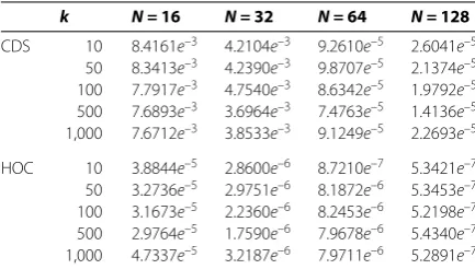
Table 1 The number of multigrid V-cycles with two schemes and different values of
k= 10, 50, 100, 500, 1,000 andλ= –0.9 for Example 1, wheree–5= 10–5
k N = 16 N = 32 N = 64 N = 128
CDS 10 3.4623e–5 2.4504e–5 2.1089e–5 3.2161e–5
50 2.7134e–5 2.3692e–5 1.9880e–5 1.7322e–5
100 1.7091e–5 1.6700e–5 1.4650e–5 1.3705e–5
500 1.1898e–5 1.1662e–5 1.1497e–5 1.1403e–5
1,000 1.1697e–5 1.3534e–5 1.9545e–5 1.6564e–5
HOC 10 7.2104e–5 1.1268e–5 9.9271e–6 9.3180e–7
50 5.2183e–5 1.6971e–5 9.9128e–6 9.3345e–7
100 3.6107e–5 1.6881e–5 7.5263e–6 9.2791e–7
500 2.1945e–5 1.5213e–5 7.6298e–6 8.4423e–7
1,000 4.3177e–5 2.2813e–5 2.1970e–5 9.9281e–7
Table 2 The number of multigrid V-cycles with two schemes and different values of
k= 10, 50, 100, 500, 1,000 andλ= 0.9 for Example 2, wheree–5= 10–5
k N = 16 N = 32 N = 64 N = 128
CDS 10 8.4161e–3 4.2104e–3 9.2610e–5 2.6041e–5
50 8.3413e–3 4.2390e–3 9.8707e–5 2.1374e–5
100 7.7917e–3 4.7540e–3 8.6342e–5 1.9792e–5
500 7.6893e–3 3.6964e–3 7.4763e–5 1.4136e–5
1,000 7.6712e–3 3.8533e–3 9.1249e–5 2.2693e–5
HOC 10 3.8844e–5 2.8600e–6 8.7210e–7 5.3421e–7
50 3.2736e–5 2.9751e–6 8.1872e–6 5.3453e–7
100 3.1673e–5 2.2360e–6 8.2453e–6 5.2198e–7
500 2.9764e–5 1.7590e–6 7.9678e–6 5.4340e–7
1,000 4.7337e–5 3.2187e–6 7.9711e–6 5.2891e–7
not increase. One of the important advantages of this scheme is the execution time. The computed results show that the line Gauss-Seidel method takes less CPU time than the other smoothers.
Example Consider the following elliptic PDE with the source term:
uxx+uyy+ku=f(x,y), <x< , <y< , ()
f(x,y) =k– e–xx–y( –y) + e–x; ()
the boundary conditions are given by the analytic solution, that is,
u(x,y) =e–xy( –y) –x .
This problem has a steep boundary layer alongx= ; therefore, we are using nonuniform grids along the x-axis, which are accumulating nearx= , and uniform grids along the y-axis with the following stretching function []:
xi=
i Nx
+λ
πsin
πi Nx
, yj=
j Ny
,
Table 3 The error norms and order of accuracy of the two schemes for Example 1, where
e–5= 10–5,e2,k= 10,N= 16, 32, 64, 128
N λ 162 322 642 1282 Order
CDS 0.0 6.0982e–4 4.9180e–4 9.9082e–5 7.9118e–5 0.310
–0.2 4.1044e–4 3.1322e–4 7.1160e–5 5.0032e–5 0.392
–0.4 2.5100e–4 1.7200e–4 6.7640e–5 3.9155e–5 0.545
–0.6 8.1398e–5 6.1021e–5 4.3302e–5 2.4203e–5 0.415 –0.8 5.8197e–5 5.0295e–5 3.0955e–5 1.5064e–5 0.531 –0.9 3.4623e–5 2.4504e–5 2.1089e–5 3.2161e–5 0.210
HOC 0.0 4.8122e–4 3.6113e–4 9.4102e–5 5.8410e–5 0.414 –0.2 1.1438e–4 1.0661e–4 6.3918e–5 4.1235e–5 0.101
–0.4 9.1100e–5 6.1818e–5 3.2561e–5 1.9760e–5 0.559
–0.6 7.1398e–5 4.5502e–5 1.6021e–5 6.2030e–6 0.650
–0.8 4.7341e–5 8.8061e–6 7.6660e–6 3.7210e–7 0.242
–0.9 7.2104e–5 1.1268e–5 9.9271e–6 9.3180e–7 2.677
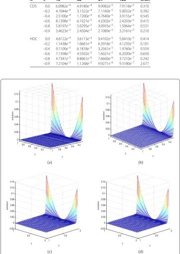
Figure 2 Computed solutions through HOC and CDS schemes for problem 1. (a)Exact solution.
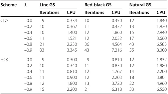
Table 4 The number of multigrid V-cycles and CPU time with two schemes and different relaxation methods with 322for Example 1
Scheme λ Line GS Red-black GS Natural GS
Iterations CPU Iterations CPU Iterations CPU
CDS 0.0 9 0.334 10 0.350 12 1.840
–0.2 10 0.362 11 0.432 13 1.920
–0.4 10 1.400 12 1.860 15 2.940
–0.6 11 1.521 12 2.032 17 3.660
–0.8 21 2.230 36 4.564 43 6.583
–0.9 33 3.345 43 7.216 55 8.000
HOC 0.0 9 0.300 9 0.810 12 1.832
–0.2 10 0.340 11 0.830 12 1.980
–0.4 11 0.810 12 1.767 14 2.200
–0.6 11 0.900 12 2.203 18 3.80
–0.8 12 1.800 13 3.720 22 4.960
–0.9 15 2.200 21 6.318 33 6.550
the boundaryx= forλ> . Ifλ= , then the grids reduced to be uniform. Whenλ= –. and the grid numbers are , the grid distribution in thexy-plane is shown in Figure .
The estimated accuracy and maximum absolute error with different stretching parameter
λare presented in Table . We see that whenλ= , the results are very poor. A more ac-curate solution and order of convergence are obtained from HOC and CD schemes with decreasing stretching parameterλon nonuniform grids. We observe that whenλ= –., the solution obtained with HOC scheme is more accurate, but whenλfurther decreases to –., the accuracy decreases. This situation is not wondering because putting more grids in the boundary layer area will necessarily cause lack of mesh points in the other regions of the domain. Figure indicates the configuration of solution in thexy-plane. Table shows thel-norm of the error, CPU timing, and the order of accuracy for
differ-ent stretching parametersλin problem . It is also obvious from the results that the line Gauss-Seidel relaxation is the most efficient smoother with the least multigrid V-cycle numbers for such type of problems. (a) shows the exact solution, (b) the solution obtained from HOC scheme on uniform grids, (c) the computed solution obtained from a HOC scheme on nonuniform grids, and (d) the computed solution of CD scheme on nonuni-form grids.
Example Consider the PDE with a source termf(x,y),
uxx+uyy+ku=f(x,y), <x,y< . ()
Its analytic solution is
u(x,y) = ( –e
(x–))( –e(y–))
( –e–) .
The source function is determined by the analytic solution with the boundary layers alongx= andy= . Hence, nonuniform grids along the coordinate directions with accu-mulation nearx= ,y= is used by the following stretching formula:
xi=
i Nx
+λ
πsin
πi Nx
Figure 3 Nonuniform grids distribution in the
xy-plane, 322,λ= 0.8.
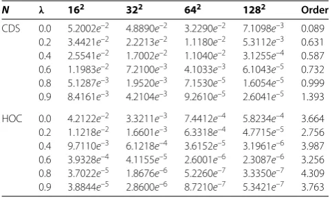
Table 5 The error norms and order of accuracy of the two schemes for Example 2, where
e–5= 10–5,e2,k= 10,N= 16, 32, 64, 128
N λ 162 322 642 1282 Order
CDS 0.0 5.2002e–2 4.8890e–2 3.2290e–2 7.1098e–3 0.089
0.2 3.4421e–2 2.2213e–2 1.1180e–2 5.3112e–3 0.631
0.4 2.5541e–2 1.7002e–2 1.1040e–2 3.1255e–4 0.587
0.6 1.1983e–2 7.2100e–3 4.1033e–3 6.1043e–5 0.732
0.8 5.1287e–3 1.9520e–3 7.1530e–5 1.6054e–5 0.999
0.9 8.4161e–3 4.2104e–3 9.2610e–5 2.6041e–5 1.393
HOC 0.0 4.2122e–2 3.3211e–3 7.4412e–4 5.8234e–4 3.664
0.2 1.1218e–2 1.6601e–3 6.3318e–4 4.7715e–5 2.756
0.4 9.7110e–3 6.1218e–4 3.6152e–5 3.1961e–6 3.987
0.6 3.9328e–4 4.1155e–5 2.6001e–6 2.3087e–6 3.256
0.8 3.7022e–5 1.8676e–6 5.2260e–7 3.3350e–7 4.309
0.9 3.8844e–5 2.8600e–6 8.7210e–7 5.3421e–7 3.763
yj=
j Ny
+ λ
πsin
πj Ny
.
Whenλgets closer to , more grids are accumulated nearx= ,y= . Whenλ= . and the grids size is , the grids distribution is given in Figure . Table indicates the
error norms and order of accuracy for different stretching parametersλfor problem . The value ofλchanges from . to .. We observe that in nonuniform grids with in-creasing the stretching parameterλ, more and more grids accumulate into the bound-ary layers; consequently, more accurate results are obtained from HOC and CD schemes. The rate of convergence continuously increases with the increase ofλ. We observe that whenλ= ., a considerably most accurate solution is obtained with the HOC scheme, but whenλincreases to ., it leads to decrease in accuracy. Figure shows the contours of the exact solution in the xy-plane. Table and Table list the number of multigrid V-cycles and the corresponding CPU time in seconds for solving problem on the ,
, , and grids. (a) represents the exact solution, (b) the solution obtained by
the HOC scheme on uniform grids, (c) the computed solution by the CD scheme on uni-form grids, and (d) the solution obtained by the HOC scheme on nonuniuni-form grids with
Figure 4 Computed solution obtained from HOC and CDS schemes for problem 2. (a)Exact solution. (b)Computed solution by HOC scheme on uniform grids.(c)CDS scheme on uniform grids.(d)HOC scheme on nonuniform grids, 322,λ= 0.8.
Table 6 The number of multigrid V-cycles and CPU time with two schemes and different relaxation methods with 322for Example 2
Scheme λ Line GS Red-black GS Natural GS
Iterations CPU Iterations CPU Iterations CPU
CDS 0.0 11 0.534 12 0.550 12 1.480
–0.2 11 0.562 12 0.630 13 1.960
–0.4 11 0.584 12 0.980 17 2.488
–0.6 12 1.765 13 1.382 19 3.600
–0.8 17 1.936 19 1.996 33 5.853
–0.9 27 3.145 33 4.162 43 6.980
HOC 0.0 9 0.310 9 0.532 12 1.330
–0.2 9 0.330 10 0.572 12 1.860
–0.4 9 0.415 11 0.677 13 2.200
–0.6 10 0.970 12 1.238 18 2.890
–0.8 11 1.770 16 1.720 22 3.973
Table 7 The number of multigrid V-cycles and CPU time with two schemes and different relaxation methods with 322for Example 2
Scheme Grids Line GS Red-black GS Natural GS
Iterations CPU Iterations CPU Iterations CPU
CDS 82 9 0.060 11 0.140 11 0.800
162 11 0.062 12 0.840 11 1.392
322 11 0.284 12 1.220 12 2.268
642 12 2.652 13 2.842 13 3.230
1282 13 2.920 15 3.296 15 3.838
HOC 82 8 0.070 8 0.532 12 0.720
162 8 0.073 8 0.660 12 0.960
322 9 0.210 9 0.977 12 1.862
642 9 2.510 10 1.322 13 2.890
1282 11 2.872 12 2.260 18 3.713
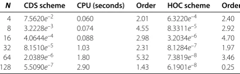
Table 8 The error norms and CPU (seconds) for a multigrid method with different discretized schemes for Example 3,e2,k= 10
N CDS scheme CPU (seconds) Order HOC scheme Order
4 7.5620e–2 0.060 2.01 6.3220e–4 2.40 8 3.2228e–3 0.074 4.55 8.3311e–5 2.92
16 4.0644e–4 0.088 2.98 3.2034e–6 4.70
32 8.1510e–5 1.03 2.31 8.1284e–7 1.97
64 2.0389e–6 1.80 5.32 7.3819e–8 3.46
128 5.5090e–7 2.90 1.43 6.1901e–8 0.25
Example Consider the Helmholtz equation with a source functionf(x,y),
uxx+uyy+ku=f(x,y), <x,y< ,
f(x,y) =
k–π
sin
πx
sin
πy
,
()
with the Dirichlet boundary condition. Its analytic solution is
u(x,y) =sin
πx
sin
πy
.
We observe that the exact solution does not show high variations; therefore, nonuniform grids are not necessary. Uniform grids are used for this problem to check the effectiveness of the multigrid method. The results obtained from the HOC and CD schemes are pre-sented. The reported error is the error norm over the discretized grid points on the finest grid level. Table lists the number of multigrid V-cycles and the corresponding CPU time in seconds for solving problem on the , , , and grids. We can see that, for this problem, the multigrid method is very efficient and all the smoothers work well.
5 Conclusion
fourth order for the HOC scheme and second order for the CD scheme. Numerical results show that the multigrid method with HOC scheme has the required accuracy and is faster than the CD scheme.
Competing interests
The authors declare that they have no competing interests.
Authors’ contributions
The authors equally contributed in the paper. All authors read and approved the final manuscript.
Author details
1Department of Mathematics, Abdul Wali Khan University, Mardan, Pakistan.2Department of Basic Sciences, University of Engineering and Technology, Peshawar, Pakistan.
Acknowledgements
The authors would like to express their gratitude to the editors and anonymous reviewers for their valuable suggestions, which substantially improved the standard of the paper.
Received: 7 June 2015 Accepted: 10 January 2016
References
1. Ge, Y, Cao, F: Multigrid method based on the transformation-free HOC scheme on nonuniform grids for 2D convection diffusion problems. J. Comput. Phys.230, 4051-4070 (2011)
2. Boisvert, RF: A fourth-order accurate Fourier method for the Helmholtz equation in three dimensions. ACM Trans. Math. Softw.13, 221-234 (1987)
3. Sutmann, G: Compact finite difference scheme of sixth order for the Helmholtz equation. J. Comput. Appl. Math.293, 15-31 (1987)
4. Singer, I, Turkel, E: High-order finite difference method for the Helmholtz equation. Comput. Methods Appl. Mech. Eng.163, 343-358 (1998)
5. Harari, I, Turkel, E: Accurate finite difference methods for time-harmonic wave propagation. J. Comput. Phys.119, 252-270 (1995)
6. Harari, I, Hughes, TJ: Finite element methods for the Helmholtz equation in an exterior domain model problem. Comput. Methods Appl. Mech. Eng.87, 59-96 (1991)
7. Mehdizadeh, O, Paraschiviou, M: Investigation of a two-dimensional spectral method for Helmholtz’s equation. J. Comput. Phys.189, 111-129 (2003)
8. Nabavi, M, Siddique, MH, Dargahi, J: Sixth-order accurate compact finite-difference method for the Helmholtz equation. J. Sound Vib.307, 972-982 (2007)
9. Brandt, A: Multi-level adaptive solution to boundary value problems technique. Math. Comput.31, 333-390 (1977) 10. Gupta, MM, Kouatchou, J, Zhang, J: A compact multigrid solver for convection-diffusion equation. J. Comput. Phys.
132, 123-129 (1997)
11. Zhang, J, Ge, L, Kouatchou, J: A two colorable fourth-order compact difference scheme and parallel iterative solution of 3D convection-diffusion equation. Math. Comput. Simul.54, 65-80 (2000)
12. Ghaffar, F, Badshah, N, Islam, S: Multigrid method for solution of 3D Helmholtz equation based on HOC schemes. Abstr. Appl. Anal.2014, Article ID 954658 (2014)
13. Ghaffar, F, Badshah, N, Khan, MA, Islam, S: Multigrid method for 2D Helmholtz equation using higher order finite difference scheme accelerated by Krylov subspace. J. Appl. Environ. Biol. Sci.4, 169-179 (2014)
14. Gupta, MM, Kouatchou, J, Zhang, J: Comparison of second and fourth order discretizations for multigrid Poisson solver. J. Comput. Phys.132, 226-232 (1997)
15. Kalnay de Rivas, E: On the use of nonuniform grids in finite-difference equations. J. Comput. Phys.10, 202-210 (1972) 16. Teilgland, R, Eliassen, JK: A multilevel mesh refinement procedure for CFD computations. Int. J. Numer. Methods
Fluids36, 519-538 (2001)
17. Zhang, J, Sun, H, Zhao, JJ: High order compact scheme with multigrid local mesh refinement procedure for convection-diffusion problems. Comput. Methods Appl. Mech. Eng.191, 4661-4674 (2002)
18. Ge, Y, Cao, F: A transformation-free HOC scheme and multigrid method for solving the 3D Poisson equation on nonuniform grids. J. Comput. Phys.234, 199-216 (2013)
19. Ge, Y: Multigrid method and fourth-order compact difference discretization scheme with unequal meshsizes for 3D Poisson equation. J. Comput. Phys.229, 6381-6391 (2010)
20. Zhang, J: Fast and high accuracy multigrid solution for three dimensional Poisson equation. J. Comput. Phys.143, 449-461 (1998)
21. Zhang, J: Multigrid method and fourth-order compact scheme for 2D Poisson equation with unequal mesh-size discretization. J. Comput. Phys.179, 170-179 (2002)
22. Hackbusch, W, Trottenberg, H: Multigrid Methods. Springer, Berlin (1982)
23. Liu, C: Multilevel adaptive methods in computational fluid dynamics. PhD thesis, University of Colorado at Denver (1989)
24. Wesseling, P: An Introduction to Multigrid Methods. Wiley, Chichester (1992)
25. Saad, Y: A flexible inner-outer preconditioned GMRES algorithm. SIAM J. Sci. Stat. Comput.14, 461-469 (1993) 26. Zhang, J: Preconditioned iterative methods and finite difference schemes for convection-diffusion. Appl. Math.
27. Ge, L, Zhang, Z: High accuracy iterative solution of convection diffusion equation with boundary layers on nonuniform grids. J. Comput. Phys.171, 560-578 (2001)