Second order numerical methods for the tempered fractional diffusion equations

(1)

R E S E A R C H

Open Access

Second-order numerical methods for the

tempered fractional diffusion equations

Zeshan Qiu

1

_{and Xuenian Cao}

1*

*_{Correspondence:}_{[email protected]} 1_{School of Mathematics and} Computational Science, Hunan Key Laboratory for Computation and Simulation in Science and Engineering, Xiangtan University, Xiangtan, P.R. China

Abstract

In this paper, a class of second-order tempered difference operators for the left and right Riemann–Liouville tempered fractional derivatives is constructed. And a class of second-order numerical methods is presented for solving the space tempered fractional diffusion equations, where the space tempered fractional derivatives are evaluated by the proposed tempered difference operators, and in the time direction is discreted by the Crank–Nicolson method. Numerical schemes are proved to be unconditionally stable and convergent with orderO(h2₊

_τ

2_{). Numerical experiments}

demonstrate the eﬀectiveness of the numerical schemes.

Keywords: Tempered fractional diﬀusion equations; Second-order tempered diﬀerence operators; Stability and convergence

1 Introduction

In recent years, many fractional models [1–18,21,22,24–27] with (tempered) fractional derivatives have been widely applied in many fields of science and technology, a lot of re-search results have been obtained. Among them, Li and Deng [14] constructed a class of second-order tempered weighted and shifted Grünwald difference operators (abbr. TWSGD) for the Riemann–Liouville tempered fractional derivatives, and then a class of second-order numerical schemes was proposed for solving a two-sided space tempered fractional diffusion equation. Numerical schemes are unconditionally stable and conver-gent with orderO(h2+τ2). Dehghan et al. [6] developed a high-order numerical scheme for the space-time tempered fractional diffusion-wave equation, the numerical scheme was proved to be unconditionally stable and convergent with orderO(h4₊_τ2_{). Qu and} Liang [18] used the Crank–Nicolson method and TWSGD method [14] to solve a class of variable-coefficient tempered fractional diffusion equations and proved that the numer-ical schemes are unconditionally stable and convergent with orderO(h2₊_τ2_{). Yu et al.} [24] extended quasi-compact discretizations to Riemann–Liouville tempered fractional derivatives and derived the numerical scheme for solving a tempered fractional diffusion equation. Yu et al. [25] constructed a numerical scheme for one-sided space tempered fractional diffusion equation, and the numerical scheme was shown to be stable and con-vergent with orderO(h3+τ).Çelik and Duman [2] solved the symmetric space tempered fractional diffusion equation by the finite element method and achieved convergence or-derO(h2₊_τ2_{). Zhang et al. [}₂₇_{] proposed a modified second-order Lubich tempered} differ-ence operator for the Riemann–Liouville tempered fractional derivatives and constructed

(2)

a numerical scheme for solving the normalized Riesz space tempered fractional diffusion equation. The stability and convergence of the numerical scheme have been proved. Hu and Cao [12] combined the implicit midpoint method and the modified second-order Lu-bich tempered difference operator to derive a numerical scheme for solving the normal-ized Riesz space tempered fractional diffusion equation with a nonlinear source term and discussed the stability and convergence of the numerical scheme.

In this paper, we consider the following space tempered fractional diﬀusion equation [14]:

⎧ ⎪ ⎪ ⎨ ⎪ ⎪ ⎩

∂u(x,t)

∂t =l ∂–α,λu(x,t)

∂xα +r ∂+α,λu(x,t)

∂xα +f(x,t), (x,t)∈(a,b)×(0,T],

u(x, 0) =ϕ(x), x∈[a,b],

u(a,t) =ψl(t), u(b,t) =ψr(t), t∈[0,T],

(1)

where 1 <α< 2 andλ≥0,f(x,t) is the linear source term, diﬀusion coeﬃcientslandrare nonnegative constants withl+r= 0, and ifl= 0, thenψl(t)≡0, ifr= 0, thenψr(t)≡0. The normalized left and right Riemann–Liouville tempered fractional derivatives∂–α,λu(x,t)

∂xα

and∂+α,λu(x,t)

∂xα are deﬁned as follows [1,14]:

∂α,λ

– u(x,t)

∂xα =aD α,λ

x u(x,t) –λ α

u(x,t) –αλα–1∂u(x,t) ∂x ,

∂α,λ

+ u(x,t)

∂xα =xD α,λ

b u(x,t) –λ

α_u₍_x_,_t_{) +}_αλα–1∂u(x,t)

∂x ,

here the left and right Riemann–Liouville tempered fractional derivativesaDαx,λu(x,t) and

xDαb,λu(x,t) are deﬁned by

aDαx,λu(x,t) =

e–λx

Γ(2 –α)

∂2

∂x2

x

a

eλτ_u₍_τ_,_t₎ (x–τ)α–1dτ

,

xDαb,λu(x,t) =

eλx

Γ(2 –α)

∂2 ∂x2

b

x

e–λτ_u₍_τ_,_t₎ (τ–x)α–1 dτ

,

whereΓ(·) is the gamma function.

Obviously, whenλ= 0, the left and right Riemann–Liouville tempered fractional deriva-tives degenerate to the left and right Riemann–Liouville fractional derivaderiva-tives, respec-tively. Whenl=r= –₂_cos1₍απ

2 ), the two-sided tempered fractional diﬀusion equation

de-generates to the normalized Riesz tempered fractional diﬀusion equation.

Considering these existing works in the literature, the aim of this paper is to try to give a class of new second-order tempered diﬀerence operators; then, using the Crank–Nicolson method and the proposed diﬀerence operators, to construct a class of second-order nu-merical methods for solving problem (1) and give the theoretical analysis of the numerical methods.

(3)

2 Second-order tempered difference operators

In this section, we ﬁrst introduce a fractional Sobolev spaceSn+α

λ (R) deﬁned as follows [27]:

Snλ+α(R) = νν∈L1(R), and

R

λ2+w2n+2α_νˆ₍_w₎_dw_<∞

, (2)

whereνˆ(w) =_Rν(x)e–iwxdxis the Fourier transform ofν(x).

Lemma 2.1([27]) Letν(x)∈L1(R), 1 <α< 2,andλ≥0.Then the Fourier transforms of the left and right Riemann–Liouville tempered fractional derivatives are

F–∞Dαx,λν

(w) = (λ+iw)ανˆ(w)

and

FxDα+,∞λν

(w) = (λ–iw)ανˆ(w).

Lemma 2.2([1,14]) Let1 <α< 2,λ≥0,the shift number p is an integer,h is the step size,

ν(x)is deﬁned on the bounded interval[a,b]and belongs to S2+α

λ (R)after zero extension

on the interval x∈(–∞,a)∪(b, +∞).The shifted Grünwald type diﬀerence operators are deﬁned as follows:

Aα_h,_,_pλν(x) = 1

hα

[x–_ha]+p

k=0

wα_ke–(k–p)λhνx– (k–p)h– 1

hαGp(1)ν(x), (3)

ˆ

Aα_h,_,_pλν(x) = 1

hα

[b–_hx]+p

k=0

wα_ke–(k–p)λhνx+ (k–p)h– 1

hαGp(1)ν(x), (4)

then

Aα_h,_,_pλν(x) =aDxα,λν(x) –λαν(x) +O(h), (5)

ˆ

Aα_h,_,_pλν(x) =xDαb,λν(x) –λ

α_ν₍_x_{) +}_O₍_h_), ₍₆₎

where wα

k= (–1)k(αk) (k≥0)denotes the normalized Grünwald weights,

Gp(s) =epλh1 –e–λhsα= +∞

k=0

wα_ke–(k–p)λhsk.

Meanwhile,denote

Wp(s) =eps

1 –e–s s

α

= 1 +

p–α 2

s+

p2

2 –

pα

2 +

α

6 +

α(α– 1) 8

s2+O|s|3

(4)

Lemma 2.3 Let1 <α< 2,λ≥0,the shift number p is an integer,h is the step size,ν(x)is

Proof Taking the Fourier transform on both sides of (7) and (8), we obtain

(5)

ˆ

φ(w) =FBˆα_h_,,_pλν(w) –FxDα+∞,λν–λ

α_ν (w)

=(λ–iw)αWˆp

(λ–iw)h– 1–λαWˆp(λh) – 1νˆ(w),

and there exist two positive constantsCandCˆ such that

φ(w)≤Ch|λ+iw|α+1+h|λ|α+1νˆ(w),

φˆ(w)≤ ˆCh|λ–iw|α+1+h|λ|α+1νˆ(w).

Taking the inverse Fourier transform of φ(w) and utilizing known conditions ν(x)∈

S2+α

λ (R), we can obtain Bα_h_,,λ_pν(x) ––∞Dαx,λν(x) +λ

α_ν

(x)≤ 1 2π

R

φ(w)dw

≤Ch

R

|λ+iw|α+1₊_|_λ_|α+1_ν_ˆ₍_w₎_dw₌_O₍_h_).

Similar provability

Bˆα_h_,,λ_pν(x)–xDα₊_∞,λν(x) +λαν(x)≤ 1 2π

R

φˆ(w)dw

≤ ˆCh

R

|λ–iw|α+1+|λ|α+1νˆ(w)dw=O(h).

The proof is completed.

Lemma 2.4 Let1 <α< 2,λ≥0,h is the step size,ν(x)is deﬁned on the bounded interval

[a,b]and belongs to S2+α

λ (R)after zero extension on the interval x∈(–∞,a)∪(b, +∞).The

new second-order tempered diﬀerence operators are given as follows:

C_hα,λν(x) =γ1Aαh,1,λν(x) +γ2Bαh,1,λν(x) +γ3Bαh,–1,λ ν(x)

= 1

hα

[x–_ha]+1

k=0

γ1wαk+γ2wˆαk+γ3wˆαk–2

e–(k–1)λhνx– (k– 1)h

– 1

hα

γ1eλh

1 –e–λhα+γ2eλh

1 –e–2λh 2

α

+γ3e–λh

1 –e–2λh 2

α

ν(x)

= 1

hα

[x–_ha]+1

k=0 gα

kν

x– (k– 1)h– 1

hαG˜1(1)ν(x), (11)

ˆ

C_hα,λν(x) =γ1Aˆαh,1,λν(x) +γ2Bˆαh,1,λν(x) +γ3Bˆαh,–1,λ ν(x)

= 1

hα

[b–_hx]+1

k=0

γ1wαk+γ2wˆαk+γ3wˆαk

e–(k–1)λhνx+ (k– 1)h

– 1

hα

γ1eλh

1 –e–λhα +γ2eλh

1 –e–2λh 2

(6)

+γ3e–λh

Proof Taking the Fourier transform on both sides of (11) and (12), we obtain

(7)

withs= (λ+iw)horλh,i2_{= –1.}

FCˆ_hα,λν(w) =γ1F

_ˆ

Aα_h_,1,λν(w) +γ2F

_ˆ

Bα_h,_,1λν(w) +γ3F

_ˆ

Bα_h_,–1,λν(w) = 1

hα

+∞

k=0

γ1wαk+γ2wˆαk+γ3wˆαk–2

e–(k–1)(λ–iw)h_ν_ˆ₍_w₎

– 1

hα

γ1eλh

1 –e–λhα+γ2eλh

1 –e–2λh 2

α

+γ3e–λh

1 –e–2λh 2

α

ˆ

ν(w)

=eh(λ–iw)

γ1

1 –e–(λ–iw)h

h

α

+γ2

1 –e–2(λ–iw)h 2h

α

ˆ

ν(w)

+γ3e–h(λ–iw)

1 –e–2(λ–iw)h 2h

α

ˆ

ν(w) –

γ1eλh

1 –e–λh

h

α

+γ2eλh

1 –e–2λh 2h

α

+γ3e–λh

1 –e–2λh 2h

α

ˆ

ν(w) =(λ–iw)αW˜(λ–iw)h–λαW˜(λh)νˆ(w),

whereW˜(s) withs= (λ–iw)horλh,i2_{= –1.} And then making

⎧ ⎨ ⎩

γ1+γ2+γ3= 1,

γ1(1 –α₂) +γ2(1 –α) +γ3(–1 –α) = 0,

we get

γ1= 2α– 2

α +

4

αγ3, γ2=

2 –α α –

4 +α α γ3.

Denote

φ(w) =FC_hα,λν(w) –F_–_∞Dα_x,λν–λαν(w)

=(λ+iw)αW˜(λ+iw)h– 1–λαW˜(λh) – 1νˆ(w),

ˆ

φ(w) =FC_hα,λν(w) –FxDα+,∞λν–λαν

(w)

=(λ–iw)αW˜(λ–iw)h– 1–λαW˜(λh) – 1νˆ(w),

and there exist two positive constantsCandCˆ such that

φ(w)≤Ch2|λ+iw|α+2+h2|λ|α+2νˆ(w),

(8)

Taking the inverse Fourier transform of φ(w) and utilizing known conditions ν(x)∈

S2+λα(R), we can obtain

Cα_h,λν(x) ––∞Dxα,λν(x) +λαν(x)≤ 1 2π

R

φ(w)dw

≤Ch2

R

|λ+iw|α+2+|λ|α+2νˆ(w)dw

=Oh2.

Similar provability

Cˆα_h,λν(x) –xDα+,∞λν(x) +λ

α_ν

(x)≤ 1 2π

R

φˆ(w)dw

≤ ˆCh2

R

|λ–iw|α+2+|λ|α+2νˆ(w)dw

=Oh2_.

In this part, because of the selectivity ofγ3, a class of approximation operators with second-order accuracy for the Riemann–Liouville tempered fractional derivatives is given.

3 Numerical schemes

For the space interval [a,b] and the time interval [0,T], we choose the grid pointsxi=

a+ih, 0≤i≤N,tn=nτ, 0≤n≤M, whereh= (b–a)/Nis the space stepsize,τ=T/M denotes the time stepsize. The exact solution and numerical solution at the point (xi,tn) are denoted byun

i =u(xi,tn) andUin, respectively. Denotingtn+1/2= (tn+tn+1)/2,fin=f(xi,tn). In this paper,u(x,·) is deﬁned on the bounded interval [a,b] andu(x,·) belongs toS2+α

λ (R) after zero extension on the intervalx∈(–∞,a)∪(b, +∞).

Using the Crank–Nicolson method to discrete time for problem (1) at point (xi,tn), we get

un+1 i –uni

τ =l

∂_–α,λu

∂xα n+1/2

i +r

∂₊α,λu

∂xα n+1/2

i

+f_in+1/2+Oτ2,

1≤i≤N– 1, 0≤n≤M– 1. (15)

From Lemma2.4, we obtain

un+1 i –uni

τ =l

Cα_h,λun_i+1/2–αλα–1δxuni+1/2

+rCˆα_h,λu_in+1/2+αλα–1δxuni+1/2

+f_in+1/2+Oτ2+h2, (16)

whereδxuni = un_i₊₁–un_i_–1

2h ,u n+1/2

(9)

Rearrange (16) to get

u_in+1–un_i =τlC_hα,λun_i+1/2+τrCˆ_hα,λun_i+1/2–τ αλα–1(l–r)δxuni+1/2

+τf_in+1/2+Oτ3+h2τ. (17)

Furthermore, (17) can be written as

un_i+1–un_i =τl 1 hα

i+1

k=0 gα

kuni–+1/2k+1–τ(l+r) 1

hαG˜(1)u n+1/2 i

+τr 1 hα

N–i+1

k=0

g_kαun_i₊+1/2_k_–1–τ αλα–1(l–r)u n+1/2 i+1 –uni–1+1/2

2h

+τf_in+1/2+Oτ3+h2τ. (18)

Eliminating the local truncation error, we obtain the numerical scheme as follows:

U_in+1–U_in=τl 1 hα

i+1

k=0

g_kαU_in_–+1/2_k₊₁–τ(l+r)1

hαG˜(1)U n+1/2 i

+τr1 hα

N–i+1

k=0

g_kαU_in₊+1/2_k_–1–τ αλα–1(l–r)U n+1/2

i+1 –Uin–1+1/2 2h

+τf_in+1/2. (19)

That is,

U_in+1=U_in+τl 1 hα

i+1

k=0 gα

k

U_in_–_k₊₁+U_in_–+1_k₊₁

2

–τ(l+r)1

hαG˜(1)

Un i +Uin+1

2 +τr

1

hα N–i+1

k=0 gα

k

U_in₊_k_–1+U_in₊+1_k_–1

2

–τ αλα–1(l–r)U n+1

i+1 +Uin+1–Uin–1+1–Uin–1

4h +τf

n+1/2

i . (20)

Furthermore, the matrix form of (20) can be written as follows:

I–τ(lA+rA T₎

2hα +

τ αλα–1₍_l_–_r₎

4h B

Un+1=

I+τ(lA+rA T₎

2hα

–τ αλ

α–1₍_l_–_r₎

4h B

Un

(10)

whereUn_{= (}_Un

4 Stability and convergence of the numerical schemes

In order to analyze the stability and convergence of the numerical schemes, we give some lemmas.

Proof It is easy to know from the expression ofwα kthat

(11)

(12)

(13)

Combining (30) and (35), and if1–₂α<γ3≤2–₄α, then

Summarizing the above relationships, we ﬁnd that if any one of the following three con-ditions is satisﬁed:

Theorem 4.1 If matrix A is deﬁned by(22),then D=A+₂AT is strictly diagonally dominant and negative deﬁnite.

Proof DenotingD=A+AT

Because the following relationships are established:

(14)

That is,

+∞

k=0 gα

k –G˜1(1) = 0. (36)

From Lemma4.2and (36), we know

N–1

j=1 di,j< 0,

–di,i> N–1

j=i

di,j, i= 1, 2, . . . ,N– 1.

Thus, matrixDis strictly diagonally dominant. Utilizing the Gershgorin theorem [23], we know that the eigenvalues of matrixDare all negative. That is, matrixDis negative deﬁnite.

Theorem 4.2 The numerical scheme(20)is unconditionally stable.

Proof DenotingM=τ(lA₂+_hrAαT)–τ αλ α–1₍_l_–_r₎

4h B, then the matrix form (21) becomes

(I–M)Un+1= (I+M)Un+τFn+1/2. (37)

Letλ(M) represent the eigenvalue of matrixM, then the eigenvalue of matrix (I–M)–1(I+

M) is1+_1–λ_λ(₍M_M)₎. BecauseM+₂MT =τ(l+r₄)(_hAα+AT)=τ₂(l_h+αr)D, from Lemma4.1and Theorem4.1, we knowλ(M) < 0, then|_1–1+_λλ(₍_MM)₎|< 1. Thus the spectral radius of matrix (I–M)–1₍_I₊_M_{) is} less than one.

Define Uh={u|u={ui}is a grid function defined on{xi=a+ih}Ni=1–1and u0= uN = 0}. And we define the corresponding discreteL2-normuL2= (h

N–1

i=1 u2i)1/2for all u∈Uh.

Lemma 4.3([14]) For matrix M in(37),there exists

(I–M)–1₂≤1, (I–M)–1(I+M)₂≤1,

where · 2denotes2-norm(spectral norm).

Theorem 4.3 The numerical scheme(20)is convergent,i.e.,there is a constant C such that

en_L

2≤C

τ2+h2, n= 1, 2, . . . ,M,

where en_{= (}_en

1,en2, . . . ,enN–1)T,eni =uni –Uin.

Proof The proof is similar [14]. Combining (18) and (19), we obtain

(15)

whereRn_{= (}_Rn

1,Rn2, . . . ,RnN–1)T, andRni =O(τ3+τh2) is the local truncation error. Equation (38) can be rewritten as

en+1= (I–M)–1(I+M)en+ (I–M)–1Rn.

By taking the Euclidean norm · 2at the same time on both sides of the upper form, we get

en₂≤(I–M)–1(I+M)en–1₂+(I–M)–1Rn–1₂ ≤(I–M)–1(I+M)₂en–1₂+(I–M)–1₂Rn–1₂.

Noting that · L2=h1/2 · 2and from Lemma4.3, we can get

en_L

2≤(I–M)

–1₍_I₊_M₎ 2e

n–1

L2+(I–M)

–1 2R

n–1 L2

≤en–1_L

2+R

n–1 L2.

Because the local truncation error is given as|Rk_i| ≤C(τ3₊_τ_h2_{), and noticing that}_e0 L2=

0, we have

en_L

2≤e

n–1 L2+R

n–1 L2≤e

n–2 L2+R

n–1 L2

≤e0_L

2+

n–1

k=0

Rk_L

2≤C

τ2+h2.

5 Numerical experiments

The observation order is deﬁned as

Order =log₂

_e

L2,h

eL2,h/2

.

We give four examples to verify the eﬀectiveness of the numerical schemes and com-pare the numerical results of our method with those of the CN-TWSGD method [14] (max{(2–_αα2)(₊₃α2_α+₊₂α–8),(1–

α)(α2+2α)

2(α2₊₃_α₊₄₎} ≤β3≤(2–α)(α

2₊₂_α_–3)

2(α2₊₃_α₊₂₎ ,β1=α₂ +β3,β2=2–₂α– 2β3) for Exam-ple2.

Example1 ([14]) Consider the initial-boundary value problem of tempered fractional dif-fusion equation

⎧ ⎪ ⎪ ⎪ ⎪ ⎪ ⎨ ⎪ ⎪ ⎪ ⎪ ⎪ ⎩

∂u(x,t)

∂t = ∂α,λ

– u(x,t)

∂xα +e–λx+t((λα–αλα+ 1)x2+α

–Γ_Γ(3+₍₃₎α)x2₊_α₍_α_{+ 2)}_λα–1_xα+1_), ₍_x_,_t₎_∈_{(0, 1)}_×_{(0, 1],} u(0,t) = 0, u(1,t) =e–λ+t_, _t_∈_{[0, 1],}

u(x, 0) =e–λx_x2+α_, _x_∈_{[0, 1],}

where 1 <α< 2.

(16)

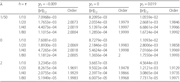
Choosing diﬀerentα,λ, andγ3, we use the proposed method to solve Example1, the errors and observation orders are displayed in Tables1,2, and3. From Tables1–3, we ﬁnd that the numerical schemes are second-order accuracy both in time and space, which is a match with theoretical results.

Table 1 Errors and corresponding observation orders att= 1,α= 1.2

λ h=τ γ3= –0.065 γ3= 0 γ3= 0.046

eL2 Order eL2 Order eL2 Order

1/50 1/10 1.3091e–03 8.9048e–03 1.5872e–02

1/20 3.4456e–04 1.9257 2.2077e–03 2.0120 3.9986e–03 1.9889 1/40 8.8261e–05 1.9649 5.4891e–04 2.0079 9.9862e–04 2.0015 1/80 2.2181e–05 1.9925 1.3688e–04 2.0037 2.4933e–04 2.0019

0 1/10 5.4687e–03 1.3477e–02 1.9237e–02

1/20 1.2413e–03 2.1393 3.2862e–03 2.0360 4.7459e–03 2.0191 1/40 2.9794e–04 2.0588 8.1182e–04 2.0172 1.1770e–03 2.0116 1/80 7.3348e–05 2.0222 2.0193e–04 2.0073 2.9313e–04 2.0055

2 1/10 3.9639e–03 8.1213e–03 1.0887e–02

1/20 9.7650e–04 2.0212 2.1455e–03 1.9204 2.9861e–03 1.8663 1/40 2.4398e–04 2.0009 5.4410e–04 1.9794 7.6695e–04 1.9611 1/80 6.1112e–05 1.9972 1.3648e–04 1.9952 1.9300e–04 1.9905

λ h=τ γ3= –0.142 γ3= 0 γ3= 0.333

eL2 Order eL2 Order eL2 Order

1/50 1/10 7.7227e–03 1.0465e–02 5.3286e–02

1/20 2.0245e–03 1.9315 2.6046e–03 2.0064 1.3526e–02 1.9780 1/40 5.1203e–04 1.9833 6.4995e–04 2.0027 3.3823e–03 1.9997 1/80 1.2836e–04 1.9960 1.6239e–04 2.0009 8.4480e–04 2.0013

0 1/10 5.7263e–03 1.1908e–02 5.3855e–02

1/20 1.5271e–03 1.9068 2.9592e–03 2.0087 1.3568e–02 1.9889 1/40 3.8755e–04 1.9783 7.3811e–04 2.0033 3.3854e–03 2.0028 1/80 9.7221e–05 1.9950 1.8439e–04 2.0011 8.4508e–04 2.0022

2 1/10 2.5444e–03 6.6079e–03 2.2144e–02

1/20 7.8955e–04 1.6882 1.7420e–03 1.9234 6.9946e–03 1.6626 1/40 2.0774e–04 1.9263 4.4145e–04 1.9804 1.8798e–03 1.8956 1/80 5.2509e–05 1.9841 1.1072e–04 1.9953 4.7865e–04 1.9735

λ h=τ γ3= –0.009 γ3= 0 γ3= 0.019

eL₂ Order eL₂ Order eL₂ Order

1/50 1/10 7.0968e–03 8.2095e–03 1.0559e–02

1/20 1.7653e–03 2.0073 2.0554e–03 1.9979 2.6681e–03 1.9846 1/40 4.4073e–04 2.0019 5.1397e–04 1.9997 6.6861e–04 1.9966 1/80 1.1015e–04 2.0004 1.2850e–04 1.9999 1.6724e–04 1.9992

0 1/10 7.6081e–03 8.7279e–03 1.1093e–02

1/20 1.8930e–03 2.0069 2.1846e–03 1.9983 2.8006e–03 1.9858 1/40 4.7265e–04 2.0018 5.4624e–04 1.9998 7.0166e–04 1.9969 1/80 1.1812e–04 2.0005 1.3656e–04 2 1.7550e–04 1.9993

2 1/10 3.2345e–03 3.6657e–03 4.5644e–03

(17)

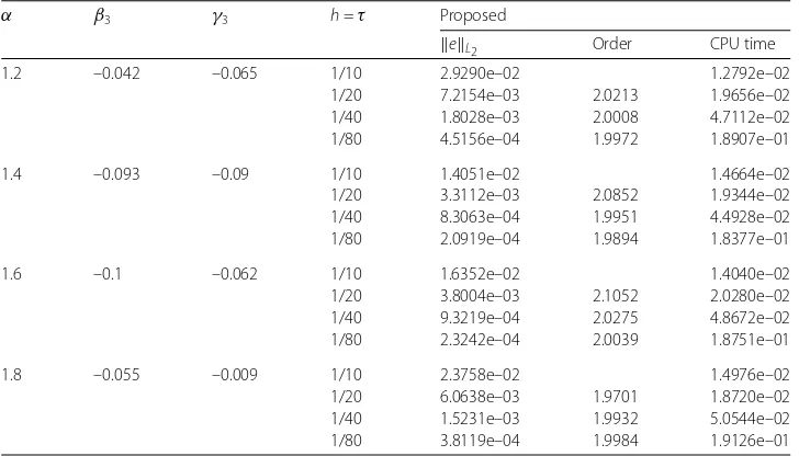
Table 4 Errors and corresponding observation orders att= 1,λ= 1/50

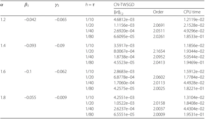
α β3 γ3 h=τ CN-TWSGD

eL2 Order CPU time

1.2 –0.042 –0.065 1/10 4.6812e–03 1.2119e–02

1/20 1.1156e–03 2.0691 2.1528e–02

1/40 2.6920e–04 2.0511 4.9296e–02

1/80 6.6095e–05 2.0261 1.8533e–01

1.4 –0.093 –0.09 1/10 3.5917e–03 1.1856e–02

1/20 8.0067e–04 2.1654 1.9344e–02

1/40 1.8738e–04 2.0952 5.0544e–02

1/80 4.5523e–05 2.0413 1.9469e–01

1.6 –0.1 –0.062 1/10 2.8683e–03 1.5912e–02

1/20 6.8778e–04 2.0602 1.7784e–02

1/40 1.7060e–04 2.0113 4.4928e–02

1/80 4.2575e–05 2.0025 1.8221e–01

1.8 –0.055 –0.009 1/10 4.2551e–03 1.3104e–02

1/20 1.0522e–03 2.0158 1.8408e–02

1/40 2.6237e–04 2.0037 4.4304e–02

1/80 6.5551e–05 2.0009 1.9531e–01

Example2 ([14]) Consider the initial-boundary value problem of tempered fractional dif-fusion equation

⎧ ⎪ ⎪ ⎪ ⎪ ⎪ ⎨ ⎪ ⎪ ⎪ ⎪ ⎪ ⎩

∂u(x,t)

∂t = ∂α+,λu(x,t)

∂xα +eλx+t((λα–αλα+ 1)(1 –x)2+α

–Γ_Γ(3+₍₃₎α)(1 –x)2₊_α₍_α_{+ 2)}_λα–1_{(1 –}_x₎α+1_), ₍_x_,_t₎_∈_{(0, 1)}_×_{(0, 1],}

u(0,t) =et_, _u_(1,_t_{) = 0,} _t_∈_{[0, 1],}

u(x, 0) =eλx_{(1 –}_x₎2+α_, _x_∈_{[0, 1],}

where 1 <α< 2.

The exact solution isu(x,t) =eλx+t_{(1 –}_x₎2+α_.

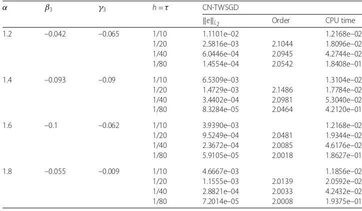
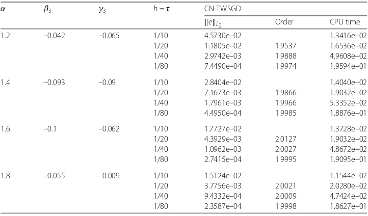
In order to compare the CN-TWSGD method with the proposed method in this paper, we choose diﬀerentα,λ,β3, andγ3 to solve Example2, the errors, observation orders, and CPU times are displayed in Tables4–9. From Tables4–9, we see that both the CN-TWSGD method and our method are eﬀective.

Example3 (cf. [27]) Consider the initial-boundary value problem of tempered fractional diﬀusion equation

⎧ ⎪ ⎪ ⎨ ⎪ ⎪ ⎩

∂u(x,t)

∂t =l ∂–α,λu(x,t)

∂xα +r ∂+α,λu(x,t)

∂xα +f(x,t), (x,t)∈(0, 1)×(0, 1],

u(0,t) = 0, u(1,t) = 0, t∈[0, 1],

u(x, 0) =e–λx_x4_{(1 –}_x₎4_, _x_∈_{[0, 1],}

where 1 <α< 2,l= 1,r= 2, and the linear source term is

f(x,t) =αeαt–λxx4(1 –x)4–eαt

e–λx 4

k=0

(–1)4_k Γ(5 +k)

(18)

Table 5 Errors and corresponding observation orders att= 1,λ= 1/50

α β3 γ3 h=τ Proposed

eL2 Order CPU time

1.2 –0.042 –0.065 1/10 1.3356e–03 1.5912e–02

1/20 3.5152e–04 1.9258 2.2152e–02

1/40 9.0044e–05 1.9649 4.8672e–02

1/80 2.2629e–05 1.9925 1.9594e–01

1.4 –0.093 –0.09 1/10 1.4612e–03 1.3728e–02

1/20 4.2047e–04 1.7971 1.9344e–02

1/40 1.0892e–04 1.9487 5.0856e–02

1/80 2.7456e–05 1.9881 2.0280e–01

1.6 –0.1 –0.062 1/10 2.2694e–03 1.2480e–02

1/20 5.0328e–04 2.1729 1.9656e–02

1/40 1.2209e–04 2.0434 5.0544e–02

1/80 3.0302e–05 2.0105 1.9313e–01

1.8 –0.055 –0.009 1/10 7.1897e–03 1.4664e–02

1/20 1.7878e–03 2.0077 2.2464e–02

1/40 4.4632e–04 2.0020 5.1480e–02

1/80 1.1154e–04 2.0005 2.0062e–01

Table 6 Errors and corresponding observation orders att= 1,λ= 0

eL2 Order CPU time

1.2 –0.042 –0.065 1/10 1.1101e–02 1.2168e–02

1/20 2.5816e–03 2.1044 1.8096e–02

1/40 6.0446e–04 2.0945 4.2744e–02

1/80 1.4554e–04 2.0542 1.8408e–01

1.4 –0.093 –0.09 1/10 6.5309e–03 1.3104e–02

1/20 1.4729e–03 2.1486 1.7784e–02

1/40 3.4402e–04 2.0981 5.3040e–02

1/80 8.3284e–05 2.0464 4.2120e–01

1.6 –0.1 –0.062 1/10 3.9390e–03 1.2168e–02

1/20 9.5249e–04 2.0481 1.9344e–02

1/40 2.3672e–04 2.0085 4.6176e–02

1/80 5.9105e–05 2.0018 1.8627e–01

1.8 –0.055 –0.009 1/10 4.6667e–03 1.1856e–02

1/20 1.1555e–03 2.0139 2.0592e–02

1/40 2.8821e–04 2.0033 4.2432e–02

1/80 7.2014e–05 2.0008 1.9375e–01

+ 2eλ(x–2) +∞

i=0 (2λ)i

i! 4

k=0

(–1)4_k Γ(5 +k+i)

Γ(5 +k+i–α)(1 –x) 4+k+i–α

– 3λαe–λx_x4_{(1 –}_x₎4₊_αλα–1_e–λx_–_λ_x4_{(1 –}_x₎4_{+ 4}_x_–_x23

(1 – 2x)

.

The exact solution isu(x,t) =eαt–λx_x4_{(1 –}_x₎4_.

(19)

eL2 Order CPU time

1.2 –0.042 –0.065 1/10 5.4687e–03 1.3728e–02

1/20 1.2413e–03 2.1393 2.2152e–02

1/40 2.9794e–04 2.0588 4.9608e–02

1/80 7.3348e–05 2.0222 1.9594e–01

1.4 –0.093 –0.09 1/10 1.4523e–03 1.3728e–02

1/20 2.8548e–04 2.3468 2.2776e–02

1/40 6.7785e–05 2.0744 4.8048e–02

1/80 1.6770e–05 2.0151 1.8876e–01

1.6 –0.1 –0.062 1/10 3.3311e–03 1.3104e–02

1/20 7.7293e–04 2.1076 1.9968e–02

1/40 1.8976e–04 2.0262 4.5240e–02

1/80 4.7234e–05 2.0063 1.9656e–01

1.8 –0.055 –0.009 1/10 7.5583e–03 1.4976e–02

1/20 1.8800e–03 2.0073 2.0904e–02

1/40 4.6938e–04 2.0019 4.8048e–02

1/80 1.1730e–04 2.0006 1.8970e–01

eL₂ Order CPU time

1.2 –0.042 –0.065 1/10 4.5730e–02 1.3416e–02

1/20 1.1805e–02 1.9537 1.6536e–02

1/40 2.9742e–03 1.9888 4.9608e–02

1/80 7.4490e–04 1.9974 1.9594e–01

1.4 –0.093 –0.09 1/10 2.8404e–02 1.4040e–02

1/20 7.1673e–03 1.9866 1.9032e–02

1/40 1.7961e–03 1.9966 5.3352e–02

1/80 4.4950e–04 1.9985 1.8876e–01

1.6 –0.1 –0.062 1/10 1.7727e–02 1.3728e–02

1/20 4.3929e–03 2.0127 1.9032e–02

1/40 1.0962e–03 2.0027 4.8672e–02

1/80 2.7415e–04 1.9995 1.9095e–01

1.8 –0.055 –0.009 1/10 1.5124e–02 1.1544e–02

1/20 3.7756e–03 2.0021 2.0280e–02

1/40 9.4332e–04 2.0009 4.7424e–02

1/80 2.3587e–04 1.9998 1.8627e–01

Example4 Consider the initial-boundary value problem of tempered fractional diﬀusion equation:

⎧ ⎪ ⎪ ⎨ ⎪ ⎪ ⎩

∂u(x,t)

∂t = ∂α_–,λu(x,t)

∂xα + ∂+α,λu(x,t)

∂xα , (x,t)∈(0, 1)×(0, 1],

u(0,t) = 0, u(1,t) = 0, t∈[0, 1],

u(x, 0) =x2_{(1 –}_x₎2_, _x_∈_{[0, 1],}

where 1 <α< 2.

(20)

eL2 Order CPU time

1.2 –0.042 –0.065 1/10 2.9290e–02 1.2792e–02

1/20 7.2154e–03 2.0213 1.9656e–02

1/40 1.8028e–03 2.0008 4.7112e–02

1/80 4.5156e–04 1.9972 1.8907e–01

1.4 –0.093 –0.09 1/10 1.4051e–02 1.4664e–02

1/20 3.3112e–03 2.0852 1.9344e–02

1/40 8.3063e–04 1.9951 4.4928e–02

1/80 2.0919e–04 1.9894 1.8377e–01

1.6 –0.1 –0.062 1/10 1.6352e–02 1.4040e–02

1/20 3.8004e–03 2.1052 2.0280e–02

1/40 9.3219e–04 2.0275 4.8672e–02

1/80 2.3242e–04 2.0039 1.8751e–01

1.8 –0.055 –0.009 1/10 2.3758e–02 1.4976e–02

1/20 6.0638e–03 1.9701 1.8720e–02

1/40 1.5231e–03 1.9932 5.0544e–02

1/80 3.8119e–04 1.9984 1.9126e–01

Table 10 Errors and corresponding observation orders att= 1,γ3= 0

α h=τ λ= 1/50 λ= 0 λ= 2

1.2 1/10 3.6036e–04 3.9643e–04 3.8557e–04

1/20 9.3836e–05 1.9412 9.8756e–05 2.0051 1.0825e–04 1.8326 1/40 2.4100e–05 1.9611 2.4944e–05 1.9852 2.7754e–05 1.9636 1/80 6.1263e–06 1.9759 6.2947e–06 1.9865 6.9556e–06 1.9964

1.5 1/10 4.8058e–04 4.9188e–04 2.3030e–04

1/20 1.2712e–04 1.9186 1.2939e–04 1.9266 6.1371e–05 1.9079 1/40 3.2771e–05 1.9557 3.3285e–05 1.9588 1.5816e–05 1.9562 1/80 8.3331e–06 1.9755 8.4560e–06 1.9768 4.0057e–06 1.9813

1.8 1/10 5.0678e–04 5.1402e–04 1.7371e–04

1/20 1.3156e–04 1.9456 1.3326e–04 1.9476 4.5103e–05 1.9454 1/40 3.3388e–05 1.9783 3.3800e–05 1.9791 1.1761e–05 1.9392 1/80 8.4106e–06 1.9890 8.5114e–06 1.9896 3.0136e–06 1.9645

Table 11 Errors and corresponding observation orders att= 1,γ3= 0

α h=τ λ= 2 λ= 3 λ= 5

1.2 1/10 4.4064e–03 7.3432e–03 1.3289e–02

1/20 1.4170e–03 1.6368 2.3874e–03 1.6210 4.6713e–03 1.5083 1/40 4.4624e–04 1.6669 7.1388e–04 1.7417 1.3593e–03 1.7810 1/80 1.4351e–04 1.6367 2.1251e–04 1.7482 3.7612e–04 1.8536

1.5 1/10 2.7871e–04 6.9236e–04 2.1027e–03

1/20 9.6202e–05 1.5346 2.3030e–04 1.5880 7.2237e–04 1.5414 1/40 3.1225e–05 1.6234 7.2323e–05 1.6710 2.3189e–04 1.6393 1/80 1.0186e–05 1.6161 2.1899e–05 1.7236 6.6164e–05 1.8093

1.8 1/10 2.6714e–04 2.7940e–04 3.2526e–04

(21)

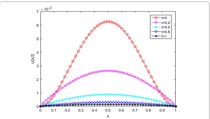
Figure 1 γ3= 0,α= 1.5,λ= 3, the change in particle concentrationu(x,t) at diﬀerent times

Figure 2 γ3= 0,α= 1.5,λ= 0, the change in particle concentrationu(x,t) at diﬀerent times

Table11. Figure1shows the particle concentration of the solution of the tempered frac-tional diffusion equation with α= 1.5 andλ= 3 at different times. Figure2 shows the particle concentration of the solution of the classical (λ= 0) fractional diffusion equa-tion withα= 1.5 at different times. It can be seen from Fig.1and Fig.2that the tem-pered fractional diffusion equation governs the transition densities, which become slower in progress.

6 Conclusion

(22)

diffusion equation. Numerical schemes are proved to be unconditionally stable and con-vergent theoretically and are verified to be effective by numerical experiments.

Acknowledgements

The authors would like to express their thanks to the anonymous referees for their valuable comments and suggestions.

Funding

This work is supported by the National Science Foundation of China (No. 11671343) and the Project of Scientiﬁc Research Fund of Hunan Provincial Science and Technology Department (No. 2018WK4006).

Availability of data and materials

The authors declare that all data and material in the paper are available and veritable.

Competing interests

The authors declare that they have no competing interests.

Authors’ contributions

Both authors contributed equally and signiﬁcantly in writing this article. Both authors wrote, read, and approved the ﬁnal manuscript.

Publisher’s Note

Springer Nature remains neutral with regard to jurisdictional claims in published maps and institutional aﬃliations.

Received: 18 May 2019 Accepted: 13 November 2019

References

1. Baeumer, B., Meerschaert, M.: Tempered stable Lévy motion and transient super-diﬀusion. J. Comput. Appl. Math. 233, 2438–2448 (2010)

2. Çelik, C., Duman, M.: Finite element method for a symmetric tempered fractional diﬀusion equation. Appl. Numer. Math.120, 270–286 (2017)

3. Dehghan, M., Abbaszadeh, M.: Spectral element technique for nonlinear fractional evolution equation, stability and convergence analysis. Appl. Numer. Math.119, 51–66 (2017)

4. Dehghan, M., Abbaszadeh, M.: An efficient technique based on finite difference/finite element method for solution of two-dimensional space/multi-time fractional Bloch–Torrey equations. Appl. Numer. Math.131, 190–206 (2018) 5. Dehghan, M., Abbaszadeh, M.: A finite difference/finite element technique with error estimate for space fractional

tempered diﬀusion-wave equation. Comput. Math. Appl.75, 2903–2914 (2018)

6. Dehghan, M., Abbaszadeh, M., Deng, W.: Fourth-order numerical method for the space-time tempered fractional diﬀusion-wave equation. Appl. Math. Lett.73, 120–127 (2017)

7. Dehghan, M., Manafian, J., Saadatmandi, A.: Solving nonlinear fractional partial differential equations using the homotopy analysis method. Numer. Methods Partial Differ. Equ.26(2), 448–479 (2010)

8. Deng, W., Zhang, Z.: Numerical schemes of the time tempered fractional Feynman–Kac equation. Comput. Math. Appl.73, 1063–1076 (2017)

9. Hanert, E., Piret, C.: A Chebyshev pseudospectral method to solve the space-time tempered fractional diﬀusion equation. SIAM J. Sci. Comput.36, A1797–A1812 (2014)

10. Heydari, M., Hooshmandasl, M., Ghaini, F., Cattani, C.: Wavelets method for the time fractional diﬀusion-wave equation. Phys. Lett. A379(3), 71–76 (2015)

11. Hooshmandasl, M., Heydari, M., Cattani, C.: Numerical solution of fractional sub-diffusion and time-fractional diffusion-wave equations via fractional-order Legendre functions. Eur. Phys. J. Plus131(8), 268 (2016) 12. Hu, D., Cao, X.: The implicit midpoint method for Riesz tempered fractional diffusion equation with a nonlinear

source term. Adv. Diﬀer. Equ.2019, 66 (2019)

13. Hu, D., Cao, X.: A fourth-order compact ADI scheme for two-dimensional Riesz space fractional nonlinear reaction–diﬀusion equation. Int. J. Comput. Math. (2019).https://doi.org/10.1080/00207160.2019.1671587

14. Li, C., Deng, W.: High order schemes for the tempered fractional diﬀusion equations. Adv. Comput. Math.42, 543–572 (2016)

15. Meerschaert, M., Sabzikar, F.: Stochastic integration for tempered fractional Brownian motion. Stoch. Process. Appl. 124, 2363–2387 (2014)

16. Moghaddam, B., Machado, J., Babaei, A.: A computationally eﬃcient method for tempered fractional diﬀerential equations with application. Comput. Appl. Math.37, 3657–3671 (2018)

17. Morgado, M., Rebelo, M.: Well-posedness and numerical approximation of tempered fractional terminal value problems. Fract. Calc. Appl. Anal.20, 1239–1262 (2017)

18. Qu, W., Liang, Y.: Stability and convergence of the Crank–Nicolson scheme for a class of variable-coefficient tempered fractional diffusion equations. Adv. Differ. Equ.2017, 108 (2017)

19. Quarteroni, A., Sacco, R., Saleri, F.: Numerical Mathematics. Springer, Berlin (2010)

20. Rall, L.: Perspectives on automatic diﬀerentiation: past, present, and future? In: Automatic Diﬀerentiation: Applications, Theory, and Implementations, pp. 1–14. Springer, Berlin (2006)

21. Sabzikar, F., Meerschaert, M., Chen, J.: Tempered fractional calculus. J. Comput. Phys.293, 14–28 (2015)

22. Sun, X., Zhao, F., Chen, S.: Numerical algorithms for the time-space tempered fractional Fokker–Planck equation. Adv. Diﬀer. Equ.2017, 259 (2017)

(23)

24. Yu, Y., Deng, W., Wu, Y.: High-order quasi-compact diﬀerence schemes for fractional diﬀusion equations. Commun. Math. Sci.15, 1183–1209 (2017)

25. Yu, Y., Deng, W., Wu, Y., Wu, J.: Third order diﬀerence schemes (without using points outside of the domain) for one sided space tempered fractional partial diﬀerential equations. Appl. Numer. Math.112, 126–145 (2017)

26. Zhang, H., Liu, F., Turner, I., Chen, S.: The numerical simulation of the tempered fractional Black–Scholes equation for European double barrier option. Appl. Math. Model.40, 5819–5834 (2016)