R E S E A R C H
Open Access
A novel improved extreme learning
machine algorithm in solving ordinary
differential equations by Legendre neural
network methods
Yunlei Yang
1, Muzhou Hou
1*and Jianshu Luo
2*Correspondence: [email protected]
1School of Mathematics and Statistics, Central South University, Changsha, China
Full list of author information is available at the end of the article
Abstract
This paper develops a Legendre neural network method (LNN) for solving linear and nonlinear ordinary differential equations (ODEs), system of ordinary differential equations (SODEs), as well as classic Emden–Fowler equations. The Legendre polynomial is chosen as a basis function of hidden neurons. A single hidden layer Legendre neural network is used to eliminate the hidden layer by expanding the input pattern using Legendre polynomials. The improved extreme learning machine (IELM) algorithm is used for network weights training when solving algebraic equation systems, and several algorithm steps are summed up. Convergence was analyzed theoretically to support the proposed method. In order to demonstrate the performance of the method, various testing problems are solved by the proposed approach. A comparative study with other approaches such as conventional methods and latest research work reported in the literature are described in detail to validate the superiority of the method. Experimental results show that the proposed Legendre network with IELM algorithm requires fewer neurons to outperform the numerical algorithm in the latest literature in terms of accuracy and execution time.
Keywords: Legendre polynomial; Legendre neural network; Improved extreme learning machine; ODEs; Classic Emden–Fowler equation
1 Introduction
Many problems encountered in science and engineering, for example, physics, chemistry, biology, mechanics, astronomy, population, resources, economics, and so on, are related to a mathematical model in the form of differential equations. Generally, the analytical ex-pressions of mathematical solutions for practical problems do not exist or are difficult to find. Therefore, it is necessary to study the numerical method of solving differential equa-tions. This means calculating approximate valueyiof exact solutiony(xi) for differential equations at discrete pointsxi,i= 0, 1, . . . in the solution domain.
For a long time, many numerical methods were proposed for solving ODEs [1], includ-ing sinclud-ingle- and multi-step methods; sinclud-ingle-step methods include Euler first order method (EM) [2], second order Runge–Kutta (R–K) method inspired by Taylor’s expansion, Suen third order R–K method (Suen-R-K3), the classic fourth-order R–K method (R-K4) [3–
5], etc. In addition, in order to obtain high accuracy, based on the numerical integration method, a lot of linear multi-step methods were proposed, such as Adams implicit for-mulas [6], methods based on Taylor expansion [7], prediction–correction algorithms [8], shooting methods [9], difference methods [10], etc. The numerical methods for solving boundary value problem (BVP) have many mature research results, with high calculation accuracy, but there is a problem that with increasing sample size, the execution time in-creases rapidly.
With the development of artificial intelligence and computer technology, more and more researchers have developed a keen interest in neural network methods. Neural networks have been used in many fields such as pattern recognition [11], graphics processing [12], risk assessment [13], control systems [14], forecasting [15–18], and classification [19], showing wide application prospects. Based on the advantages of neural network meth-ods, the use of neural network function approximation capabilities [20–22] has led to the development of a number of adopted neural network model for solving differential equa-tions. The neural network methods for solving differential equations mainly include the following categories: multilayer perceptron neural network [23–28], radial basis function neural network [29–31], multi-scale radial basis function neural network [32–35], cellular neural network [36,37], finite element neural network [38–46] and wavelet neural net-work [28]. The main research focuses on two parts: the construction of the approximate solution and the weights training algorithm.
Approximate solutions of differential equations are often constructed by selecting dif-ferent activation functions: Meade and Fernandez [47,48] used a hard limit function as an activation function to construct the neural network model; Lagaris and Likas [23] pro-posed that multi-layer perceptrons can be used to construct approximate solutions; a hy-brid technique for constructing the neural network was studied by Ioannis and Tsoulos [49]; Mall and Chakraverty [50] used a Legendre polynomial as an activation function to construct an approximate solution; Xu Liying, Wen Hui and Zeng Zhezhao [51] proposed using a triangular basis function as an activation function to construct approximate solu-tions for solving ODEs. Regarding the research on network weights training optimization algorithm, we mention Reidmiller and Braun [52] who proposed RPROP algorithm based on local adaptation; Lagaris and Likas [23] proposed using DE-evolutionary algorithm to train the weights in the neural network model of partial differential equations; Malek and Shekari Beidokhti [53] presented an optimization algorithm for hybrid neural network model; Rudd and Ferrari [54] analyzed the constrained integral method (CINT) combin-ing the classical Galerkin method with the constrained BP process; Lucie and Peter [55] proposed genetic algorithms for solving a neural network model.
The aim and motivation of the present method is to propose a new Legendre neural network with IELM algorithm to solve differential equations such as linear or nonlinear ordinary differential equations, system of ordinary differential equations, and singular ini-tial value Emden–Fowler equations. IELM algorithm is used here for training the network weights. The advantages of the proposed approach are as follows:
• It is a single hidden layer neural network—by randomly choosing of the input layer weights, we only need to train the weights of the output layer.
• It is easy to implement and runs quickly.
• The improved extreme learning machine algorithm is an unsupervised learning algorithm, and we use no optimization technique.
• Calculation accuracy is higher than for other numerical methods presented in the recent literature.
The organization of this paper is as follows: we give a description of the problem to be solved in the next section. Section 3talks about constructing Legendre neural net-work for approximating and solving ODEs. IELM algorithm for training netnet-work weights is proposed and several algorithm steps are summed up in Sect.4. In Sect.5, convergence analysis of the proposed Legendre network is verified. We provide many numerical results to verify the effectiveness of the algorithm and its superiority in performance in Sect.6. Finally, in Sect.7we present some conclusions and directions for future research.
2 Description of the problem
We first introduce the general form of the following ordinary differential equations.
2.1 Second-order ordinary differential equations
We usually describe two-point BVP of second-order ODEs in the following form: ⎧
⎨ ⎩
y=f(x,y,y),
y(a) =α1, y(b) =α2,
a≤x≤b. (1)
2.2 First-order system of ordinary differential equations Let us use the following formula to represent the first-order SODE:
⎧ ⎨ ⎩
yi=fi(x,y1,y2, . . . ,yn, )
yi(a) =αi,
a≤x≤b(i= 0, 1, . . . ,n). (2)
We know that first-order ODEs is a particular case of a system of ordinary differential equations (2).
2.3 Higher-order ODEs and higher-order SODE problem Higher-order ODEs have the general form as below:
⎧ ⎨ ⎩
y(n)=f(x,y,y,y, . . . ,y(n–1)),
y(a) =α0, y(a) =α1, . . . ,y(n–1)(a) =αn–1,
If we make the transformation y1 =y,y2 =y, . . . ,yn =y(n–1), the higher-order ODEs change to the following SODE:
⎧ If for a higher-order SODE composed of two higher-order ODEs
⎧ then the above system of higher-order ODEs can be expressed as:
⎧
Considering the same notation as that of Jose [56], we can describe the above linear or nonlinear ordinary differential equations in the following general form:
Ly(x) = f(x) inI (7)
with the initial or boundary conditions
By(x) =α on∂I, (8)
By established the ODEs problem, differential equations (7) and (8) can be transformed into a constrained optimization problem in the following form:
minimize
3 Legendre basis function neural network for approximating and solving ODEs 3.1 Legendre basis function neural networks and approximation
In this subsection, employing the recursive properties of Legendre polynomials, we will discuss construction of approximate solutions based on Legendre basis function neural network.
Theorem 1 Suppose that the vectorP(x)is defined asP(x) = [P0(x),P1(x), . . . ,PN+1(x)],in
which Pn(x),n= 0, 1, . . . ,N+ 1is the nth order Legendre polynomial in the interval[0, 1],
and letP(x)be defined asP(x) = [P0(x),P1(x), . . . ,PN+1(x)],where Pn(x),n= 0, 1, . . . ,N+ 1
is the derivative of the nth order Legendre polynomial Pn(x).ThenP(x) = P(x)M,whereM
is the Legendre operational matrix given by
M=
Proof The derivatives of Legendre polynomials satisfy the recurrence relation
Pn+1(x) –Pn–1(x) = (2n+ 1)Pn(x), (11)
and from this property, we can easily draw the conclusion.
Theorem 2 For any continuous function y: [a,b]→R,there is a natural number N, con-stants an,bn,βn(n= 0, 1, . . . ,N),and Legendre polynomials P0(x),P1(x), . . . ,Pn(x),such that
the Legendre neural network with N+ 1neurons is given by
yLNN(x) = N
n=0
βnPn(anx+bn), (12)
yLNNis an approximation of y,and
3.2 Legendre basis function neural networks for solving ODEs
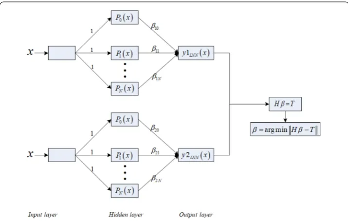
Legendre basis neural networks consist of three layers: an input layer, a hidden Legendre basis function layer and an output layer. The output of Legendre basis neural network for general differential problem described in (7) is as follows:
yLNN(x) = hidden node,βis the hidden layer-to-output layer weight vector.
Substituting the approximate solution (14) into (7) and boundary conditions (8), we can obtain an equation system of weightsβ, and the new equation system is
LyLNN(x) = f(x) inI,
ByLNN(x) =α on∂I.
(15)
Using a discretization of intervalI={xi:xi∈I,i= 0, 1, . . . ,M}, define fi= f(xi). Then the weightsan,bn,βcan be solved for from the following system of equations:
⎡
Let us take the following SODE as an example: ⎧
Noting thatxi=a+bM–ai,i= 0, 1, . . . ,M, and defining
we can rewrite equation (20) in the form:
Hβ= T. (21)
By solving the new system equation (21), the unknown weights of the Legendre neural network are obtained.
Generally, by using the Legendre basis function neural network, the approximate solu-tion of ODEs can be constructed. Then substituting the true solusolu-tion of the problem by the approximate solution and its derivatives, we can obtain a system equation for finding network weights; the process is shown in Fig.1.
4 IELM algorithm for training the Legendre neural networks
There are many numerical algorithms for solving system equation (21). In this paper, fol-lowing the ELM algorithm proposed by Huang Guangbin [57], we use IELM algorithm to train the Legendre network.
Theorem 3 The system equationHβ= Tis solvable in the following several cases: (I) If matrixHis a square invertible matrix,thenβ= H–1T.
(II) If matrixHis rectangular,thenβ= H†T,andβis the minimal least-squares solution ofHβ= T,that is,β=arg minHβ– T.
(III) IfHis a singular matrix,thenβ= H†T,andH†= HT(λI+ HHT)–1,λis regularization coefficient,which can be set according to a specific instance.
Proof For the proof of the theorem we refer to the related facts about the generalized inverse matrix in matrix theory [58] and the paper by Guang-Bin Huang [57].
Figure 1Neural network model for SODE based on Legendre polynomial
solving Hβ= T, the number of hidden neuron nodes must be less than or equal to the sample size, that is,N≤M.
But by matrix analysis theory, if matrix H is rectangular, there exists aβ, such that it is the minimal least-squares solution of Hβ= T, that is,β=arg minHβ– T. Here, H is a rectangular matrix, and the number of hidden neuron nodes does not have to be less than or equal to the sample size; we call this improved algorithm for solving Hβ= T the improved extreme learning machine (IELM).
The steps for solving ODEs using Legendre network and IELM algorithm are as follows: Step 1. Discretize the domain asa=x0<x1<· · ·<xM=b,xi=a+bM–ai,i= 0, 1, . . . ,M, and construct an approximate solution by using Legendre polynomial as an activation function, that is,yLNN(x) =Nn=0βnPn(x);
Step 2. At discrete points, substitute the approximate solutionyLNN(x) and its derivatives into the differential equation and its boundary conditions, and obtain the system equation Hβ= T;
Step 3. Solve the system equation Hβ= T by IELM algorithm introduced in Theorem3, and obtain the network weightsβ= H†T,β=arg minHβ– T;
Step 4. Form the approximate solution asyLNN(x) = N
n=0βnPn(x) = P(x)β.
5 Convergence analysis
In this section, we will verify the feasibility and convergence of the LNN method in solving differential equations by proving another theorem.
Theorem 4 Given a standard single layer feedforward neural network with n+ 1hidden nodes and Legendre basis function Pi(x) :R→R,i= 0, 1, . . . ,n,suppose that the
approx-imate solution of one-dimensional differential equations is given by(14).If we have any m+ 1distinct samples(x, f),for any an,bnrandomly chosen from any intervals of R,
Proof According to Legendre network, for anym+ 1 arbitrary and distinct samples (x, f), with x = [x0, . . . ,xm]T, f = [f0, . . . ,fm]T, let us consider the (i+ 1)th column of the Legendre hidden layer output matrix c(bi), c(bi)∈Rm+1, and suppose thatbi∈I, whereIis an open interval ofR, and
c(bi) =Pi(aix0+bi),Pi(aix1+bi), . . . ,Pi(aixm+bi) T
, (22)
then following the proof of Huang Guangbin [57], we can easily prove by contradiction that the vector c does not belong to any subspace whose dimension less thanm+ 1.
We assume thataiis generated randomly based on a continuous probability distribu-tion, for anyk=k, and we haveaixk=aixk. Suppose that c belongs to anm-dimensional subspace and vectorαis perpendicular to this subspace. Then we have
α, c(bi) – c(a)=α0·Pi(d0+bi) +α1·Pi(d1+bi) +· · ·
+αm·Pi(dm+bi) –c= 0, (23)
wheredk=aixk,k= 0, 1, . . . ,mandc=α·c(a), so we may as well assumeαm= 0, and (23) can be rewritten as
Pi(dm+bi) = – m–1
k=0
γkPi(dk+bi) +c/αm, (24)
whereγk=αk/αm,k= 0, . . . ,m– 1, by the infinite differentiability of the function on the left-hand side of (24). Calculating the derivatives ofbion both sides, we obtain
P(il)(dm+bi) = – m–1
k=0
γkP(il)(dk+bi), l= 1, . . . ,m,m+ 1, . . . , (25)
where the number of coefficientsγkis less than the number of equationsl, which produces a contradiction, and so c does not belong to any subspace whose dimension less thanm+ 1. This means that for anyan,bnrandomly chosen from any intervals ofR, such asan= 1,bn= 0, according to any continuous probability distribution, the column vectors of H can be made of full rank with probability one, which validates the above theorem.
Moreover, there exists ann≤m, so that matrix H is rectangular, and given any small positive valueε> 0 and Legendre activation functionPi(x) :R→R, formarbitrary distinct samples (x, f), and for anyan,bnrandomly chosen from any intervals ofR, according to any continuous probability distribution, we haveHm×nβn×1– fm×1<ε.
6 Numerical results and comparative study
Legendre neural network with IELM algorithm and will show that this method is very en-couraging at the end of this section.
All numerical results are obtained using MATLAB R2015a, on a computer with INTEL Core I7-6500U CPU, 4 GB of memory, 512 GB SSD and WIN10 operating system.
We use mean absolute deviation (MAD) to measure the error of numerical solution:
MAD = 1
m(1 +2 +· · ·+m), (26)
where1,2, . . . ,mis the absolute error at each discrete point.
6.1 Experimental results
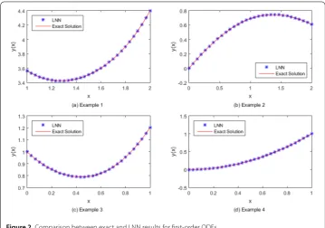
Example1 First, we consider the initial value problem of ODEs expressed as
y+cos(x)
sin(x)y= 1
sin(x),
y(1) = 3
sin(1).
This problem has been solved in [1, 2], and the exact solution isy(x) =sin(x+2)(x).
Example2 The second problem is given by
y+1 5y=e
–x5cos(x),
y(0) = 0
and considered on the interval [0, 2]. The exact solution isy(x) =e–x5sin(x).
Example3 For the third problem, we consider
y+
x+ 1 + 3x 2
1 +x+x3
y=x3+ 2x+ x 2+ 3x4 1 +x+x3,
y(0) = 1,
which has the exact solutiony(x) = e–
x2 2
1+x+x3 +x2on the interval [0, 1].
Example4 The last initial value problem of ODEs is as below:
y–sin(x)y= 2x–x2sin(x),
y(0) = 0.
It has been solved in [0, 1], with the exact solution beingy(x) =x2.
Figure 2Comparison between exact and LNN results for first-order ODEs
Figure 3The absolute error for first-order ODEs
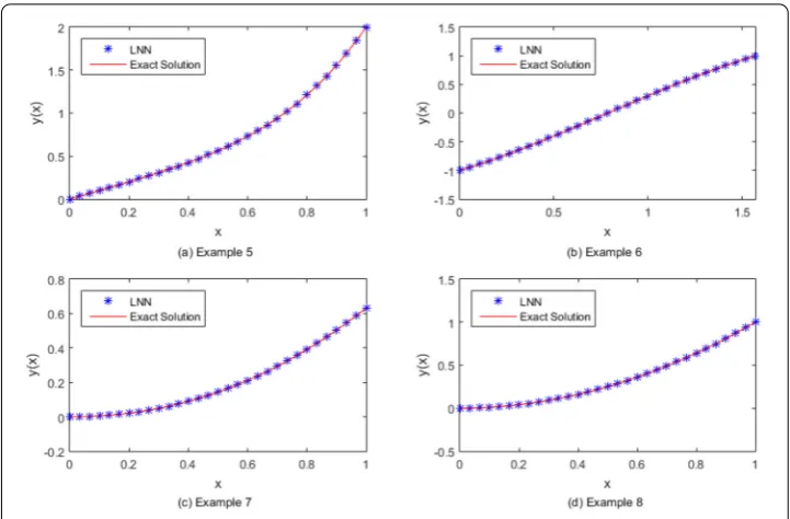
Example5 Here we consider the second-order ODEs given as follows:
y+xy– 4y= 12x2– 3x,
y(0) = 0, y(1) = 2
Figure 4Comparison between exact and LNN results for second-order ODEs
Example6 The next problem is given by
y–y= –2sin(x),
y(0) = –1, y
π
2
= 1
and considered on the interval [0,π2], with the exact solution beingy(x) =sin(x) –cos(x).
Example7 One more problem to be solved is
y+ 2y+y=x2+ 3x+ 1,
y(0) = 0, y(1) = –e–1+ 1,
which is considered on the interval [0, 1], and the exact solution isy(x) = –e(–x)+x2–x+ 1.
Example8 As the last problem we consider the following problem:
y+1 5y
+y= –1 5e
–x5cos(x),
y(0) = 0, y(2) =e–25sin(2),
defined on the interval [0, 2] and having the exact solutiony(x) =e–x5sin(x).
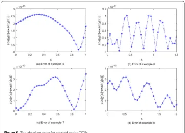
Figure 5The absolute error for second-order ODEs
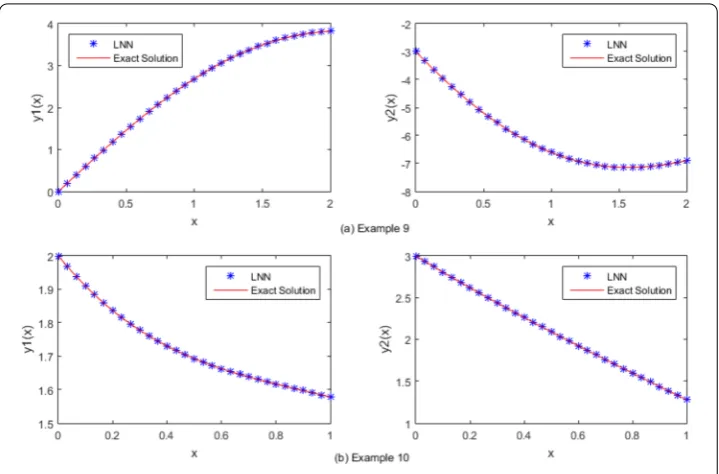
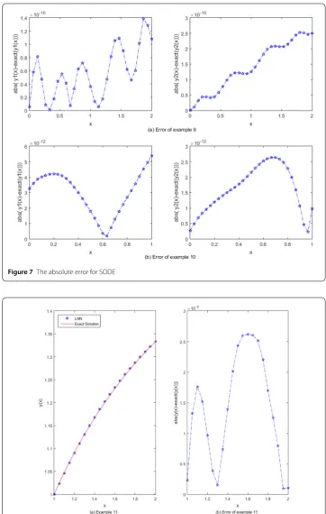
Example9 Next we consider the initial value problem of SODEs expressed as
y1+ 2y1+y2=sin(x),
y2– 4y1– 2y2=cos(x),
y1(0) = 0, y2(0) = –3,
which has been solved in [0, 2], and the exact solution is ⎧
⎨ ⎩
y1(x) = 2sin(x) +x,
y2(x) = –3sin(x) – 2cos(x) – 2x– 1.
Example10 One more problem is given by
y1+ 2y1–y2= 2sin(x),
y2–y1+ 2y2= 2
cos(x) –sin(x),
y1(0) = 2, y2(0) = 3,
and it is defined on the interval [0, 2], with the exact solution being ⎧
⎨ ⎩
y1(x) = 2e–x+sin(x),
y2(x) = 2e–x+cos(x).
Figure 6Comparison between exact and LNN results for SODE
Example11 Consider the nonlinear boundary value problem from [59]
y= 1 2x2
y3– 2y2,
y(1) = 1, y(2) = 4/3
with the exact solutiony(x) = 2x/(x+ 1).
Figure8shows the numerical solutions and absolute errors of Example11. These nu-merical results are obtained withn= 22,m= 20.
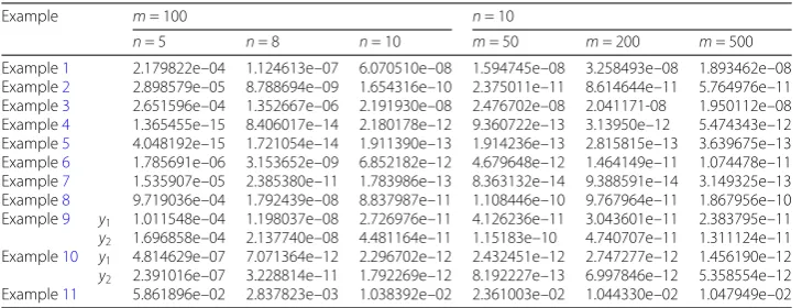
We also calculated all the test examples with different parameters. Tables1and2show the mean absolute deviation and execution time of each example. The execution time in Table2is the average time of 100 repetitions (in seconds). By analyzing the data of Tables1
and2, the best parameter value for each testing problem becomes evident, and we observe that the execution time was only slightly affected by changing network parameters.
6.2 Comparative study
A comparative study with other approaches such as traditional methods and latest re-search work is described in this subsection to verify the superiority of the proposed method. We first compared our approach with some common traditional methods.
For test Examples1–4, different methods such as Euler method (EM), Suen third-order Runge–Kutta method (Suen-R-K3),classical fourth-order Runge–Kutta method (R-K4), cosine basis function neural network based on gradient descent algorithm (CNN(GD)) and improved extreme learning machine algorithm (CNN(IELM)) were used. Tables3
Figure 7The absolute error for SODE
Figure 8(a) Comparison between exact and LNN results; (b) Absolute errors of Example11
Table 1 Mean absolute deviation of test examples with different parameters
Example m= 100 n= 10
n= 5 n= 8 n= 10 m= 50 m= 200 m= 500
Example1 2.179822e–04 1.124613e–07 6.070510e–08 1.594745e–08 3.258493e–08 1.893462e–08 Example2 2.898579e–05 8.788694e–09 1.654316e–10 2.375011e–11 8.614644e–11 5.764976e–11 Example3 2.651596e–04 1.352667e–06 2.191930e–08 2.476702e–08 2.041171-08 1.950112e–08 Example4 1.365455e–15 8.406017e–14 2.180178e–12 9.360722e–13 3.13950e–12 5.474343e–12 Example5 4.048192e–15 1.721054e–14 1.911390e–13 1.914236e–13 2.815815e–13 3.639675e–13 Example6 1.785691e–06 3.153652e–09 6.852182e–12 4.679648e–12 1.464149e–11 1.074478e–11 Example7 1.535907e–05 2.385380e–11 1.783986e–13 8.363132e–14 9.388591e–14 3.149325e–13 Example8 9.719036e–04 1.792439e–08 8.837987e–11 1.108446e–10 9.767964e–11 1.867956e–10 Example9 y1 1.011548e–04 1.198037e–08 2.726976e–11 4.126236e–11 3.043601e–11 2.383795e–11
y2 1.696858e–04 2.137740e–08 4.481164e–11 1.15183e–10 4.740707e–11 1.311124e–11 Example10 y1 4.814629e–07 7.071364e–12 2.296702e–12 2.432451e–12 2.747277e–12 1.456190e–12 y2 2.391016e–07 3.228814e–11 1.792269e–12 8.192227e–13 6.997846e–12 5.358554e–12 Example11 5.861896e–02 2.837823e–03 1.038392e–02 2.361003e–02 1.044330e–02 1.047949e–02
Table 2 Execution time of test examples with different parameters
Example m= 100 n= 10
n= 5 n= 8 n= 10 m= 50 m= 200 m= 500
Example1 0.0068 0.0073 0.0073 0.0073 0.0073 0.0077
Example2 0.0057 0.0059 0.0065 0.0063 0.0063 0.0064
Example3 0.0056 0.0059 0.0061 0.0060 0.0062 0.0068
Example4 0.0037 0.0040 0.0040 0.0041 0.0042 0.0048
Example5 0.0060 0.0063 0.0066 0.0063 0.0064 0.0071
Example6 0.0056 0.0063 0.0062 0.0062 0.0061 0.0067
Example7 0.0058 0.0059 0.0062 0.0060 0.0063 0.0067
Example8 0.0057 0.0060 0.0061 0.0060 0.0062 0.0075
Example9 0.0120 0.0121 0.0121 0.0122 0.0124 0.0132
Example10 0.0118 0.0112 0.0114 0.0113 0.0117 0.0123
Example11 0.0025 0.0030 0.0037 0.0033 0.0049 0.0082
Table 3 Mean absolute deviation of different methods for first-order ODEs
ODEs EM Suen-R-K3 R-K4 CNN(GD) CNN(IELM) LNN
Example1 0.009438 7.199659e–08 3.516257e–11 3.038010e–04 0.018023 6.070510e–08 Example2 0.006143 2.556570e–08 2.508454e–11 5.306315e–04 0.010317 1.654316e–10 Example3 0.003830 6.992166e–08 4.140991e–10 2.502357e–04 0.007621 2.191930e–08 Example4 0.005874 4.650619e–09 2.364301e–11 2.463780e–04 0.010018 2.180179e–12
Table 4 Execution time of different methods for first-order ODEs
ODEs EM Suen-R-K3 R-K4 CNN(GD) CNN(IELM) LNN
Example1 1.4122 4.3523 5.7430 57.2749 0.0311 0.0056
Example2 1.4694 4.1127 5.8199 3.6168 0.0315 0.0106
Example3 1.3024 3.9871 5.2435 75.1474 0.0268 0.0063
Example4 1.2431 3.9994 5.3399 46.1268 0.0272 0.0043
execution time are shown in Tables6and7. It is tempting to conclude that LNN method has maximum accuracy, its execution time is less than that of the shooting and CNN (IELM) methods, and the difference is not significant with the difference method.
Table 5 Parameters of different methods
Methods Neurons (n) Sample size (m) Iterations Error sum (ε) Moment (λ)
EM – 100 100 – –
Suen-R-K3 – 100 100 – –
R-K4 – 100 100 – –
CNN(GD) 10 100 – 0.01 0.5
CNN(IELM) 10 100 – – –
LNN 10 100 – – –
Table 6 Mean absolute deviation of different methods for second-order ODEs
ODEs SM DM CNN (IELM) LNN
Example5 3.630769e–10 1.838151e–05 0.004091 1.911390e–13
Example6 5.590491e–11 1.046468e–05 0.004280 6.852182e–12
Example7 1.794887e–11 1.282581e–06 0.003461 1.783986e–13
Example8 1.110794e–09 1.439213e–05 0.001528 8.837987e–11
Table 7 Execution time of different methods for second-order ODEs
ODEs SM DM CNN(IELM) LNN
Example5 0.0375 0.0060 0.0299 0.0064
Example6 0.0365 0.0052 0.0330 0.0056
Example7 0.0372 0.0051 0.0339 0.0057
Example8 0.0371 0.0051 0.0294 0.0059
Table 8 Mean absolute deviation of different methods for SODE
ODEs EM R-K4 CNN(IELM) LNN
Example9 y1 0.018838 2.247437e–10 0.005677 2.726976e–11
y2 0.046376 5.494596e–10 0.021612 4.481164e–11
Example10 y1 0.001791 1.411037e–10 0.003651 2.296702e–12
y2 0.001202 1.041297e–10 0.006159 1.792269e–12
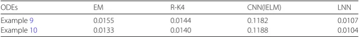
Table 9 Execution time of different methods for SODE
ODEs EM R-K4 CNN(IELM) LNN
Example9 0.0155 0.0144 0.1182 0.0107
Example10 0.0133 0.0140 0.1188 0.0104
The execution time for each algorithm in Table4is the average time of 30 repetitions, while in Tables7and9, we averaged over 100 times (results are in seconds).
By comparing with traditional methods, we testified the superiority of the new method both in terms of calculation accuracy and execution time. In order to further prove the superiority of the proposed method, a comparison with the latest reported methods is done. The following three ODEs chosen for testing the proposed method are boundary problems.
Example12 The first problem chosen from [51] is
y=y–x2+ 1,
y(0) = 0.5
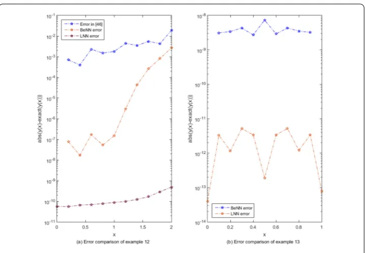
Figure 9Error comparison of Examples12and13
In our numerical experiment, the sampling parameter ism= 10, the result is shown in Fig.9(a). By comparison, the maximum error in [51] is 1.9e–2, the maximum error of BeNN method in [60] is 2.7e–3, and the maximum error of the proposed LNN method is 4.9e–10. It is easy to seen from Fig.9(a) that LNN method can obtain higher solution accuracy than the other two, which fully validates the superiority of LNN method with IELM algorithm.
Example13 The second differential equation is given by [61]
y+y= 2,
y(0) = 1,y(1) = 0
with the exact solution beingy(x) = cossin(1)–2(1) sin(x) –cos(x) + 2,x∈[0, 1].
The sampling parameter in this test experiment ism= 10, the result is shown in Fig.9(b). By comparison, the maximum error of BeNN method in [60] is 7.3e–9, and the maximum error of the proposed LNN method is 5.2e–12, so it is easy to seen from Fig.9(b) that LNN method can obtain higher accuracy solution than BeNN method in [60]. Considering the method given by [61], the maximum error is 3.5e–2 withm= 50, while, using LNN method, we are able to obtain a higher accuracy with maximum error 2.4e–13 byn= 10 neurons, which also fully validates the superiority of LNN method with IELM algorithm.
Example14 We also test the SODE given by [49]
y1=cos(x), y1(0) = 0,
Figure 10 Comparison between exact and LNN results of Example14
y3=y2, y3(0) = 0,
y4= –y3, y4(0) = 1,
y5=y4, y5(0) = 0
and its exact solution y1(x) =sin(x),y2(x) =cos(x),y3(x) = sin(x),y4(x) = cos(x),y5(x) =
sin(x),x∈[0, 1].
As shown in Figs.10and11, the sampling parameter ism= 10 in this study, and only withn= 9 neurons. By comparison with the method proposed in [49] and BeNN method in [60], the maximum errors are 2.3e–5 and 6.8e–8, the obtained maximum error of LNN method with IELM algorithm is 4.0e–12, which fully validates the superiority of the new proposed method.
6.3 Classic Emden–Fowler equation
Many problems in science and engineering can be modelled by Emden–Fowler equation. A lot of attention has been focused on the numerical solution of Emden–Fowler type equa-tion. In this subsection, we will apply the proposed alternative approach of Legendre neu-ral network (LNN) with IELM algorithm to solve classic Emden–Fowler equation.
Example15 Let us consider the classic Emden–Fowler equation given by [62]
y+2
xy
+ 2y= 0,
Figure 11 The absolute error of Example14
where the exact solution isy=sin √
2x √
2x ,x∈[0, 1].
Here we choose 10 equidistant points in the domain [0, 1] to train the proposed Legendre network and with 12 neurons. Figure12shows a comparison between the exact solution and LNN results, and the absolute error at each point. Table10provides a more intuitive comparison of the exact and numerical solution.
7 Conclusions
In this paper, we have presented a novel Legendre neural network to solve several linear or nonlinear ODEs. A Legendre polynomial was chosen as a basis function of the hidden neurons. We used Legendre polynomials to eliminate the hidden layer of the network by expanding the input pattern. An improved extreme learning machine (IELM) algorithm was used for network weights training when solving the algebraic equation systems. Con-vergence analysis has proved the feasibility of this method. The accuracy of the proposed method has been examined by solving a lot of testing examples, and the results obtained by the proposed method have been compared with the exact solution. We found the pre-sented method to be better. A comparative study has fully validated the superiority of the new proposed method over other numerical algorithms published in the latest literature. An application of the approach to solve the classic Emden–Fowler equation also shows the feasibility and applicability of our method. From the presented investigation we can see that the LNN neural network with IELM algorithm is straightforward, easily imple-mentable and has higher accuracy when solving ODEs.
stud-Figure 12 (a) Comparison between exact and LNN results; (b) absolute error of Example15
Table 10 Exact and LNN neural network results
Input pointsxk Exact results LNN results Absolute error
0 1 1 0
0.1 0.9966699984131 0.9966699984129 1.8e–13
0.2 0.9867198985254 0.9867198985252 2.2e–13
0.3 0.9702688457452 0.9702688457450 2.3e–13
0.4 0.9475135272247 0.9475135272245 2.3e–13
0.5 0.9187253698655 0.9187253698653 2.3e–13
0.6 0.8842466786034 0.8842466786032 2.2e–13
0.7 0.8444857748514 0.8444857748511 2.2e–13
0.8 0.7999112103978 0.7999112103976 2.1e–13
0.9 0.7510451462491 0.7510451462489 2.0e–13
1 0.6984559986366 0.6984559986364 1.8e–13
ied using neural network method to solve several fractional differential equations (FDEs). We have never dealt with the numerical solution of FDEs using neural network method. This will become an important research direction for us in the future. As mentioned in many articles, a variety of phenomena in astrophysics and mathematical physics can be described by Emden–Fowler equations, so this differential equation will also become a research direction for us in the future. If we consider only one type of orthogonal poly-nomial, there are some published papers as [67,68], hybrid methods may also be a new research direction.
Acknowledgements
The authors sincerely thank the reviewers for their careful reading and valuable comments, which improved the quality of this paper.
Funding
Competing interests
The authors declare that they have no competing interests.
Authors’ contributions
All authors contributed to the draft of the manuscript, all authors read and approved the final manuscript.
Author details
1School of Mathematics and Statistics, Central South University, Changsha, China.2College of Arts and Science, National
University of Defense Technology, Changsha, China.
Publisher’s Note
Springer Nature remains neutral with regard to jurisdictional claims in published maps and institutional affiliations.
Received: 13 September 2018 Accepted: 9 December 2018
References
1. Han, X.: Numerical Analysis. Higher Education Press, Beijing (2011) (in Chinese)
2. Zhang, Q.: Single-step method for solving the initial value problem of ordinary differential equations. Bull. Sci. Tech. 28(2), 7–9 (2012)
3. Wang, B.: Numerical solution of differential equations and Matlab implementation. J. Tongling Vocat. Tech. Coll.10(3), 95–97 (2011)
4. Wang, P., Yuan, H., Liu, P., et al.: Finite difference method and implicit Runge–Kutta method for solving Burgers equation. J. Changchun Univ. Sci. Technol.36(1), 158–160 (2013)
5. Deng, C., Dai, Z., Jiang, S.: Higher-order explicit index Runge–Kutta method. J. Beijing Univ. Chem. Technol.40(5), 123–127 (2013)
6. Li, M., Chen, H., Zhang, Z. Fifth-order Adams scheme for solving first order ODEs. J. Shaoguan Univ.34(12), 14–17 (2013)
7. Huang, Z., Hu, Z., Wang, C..: A study on construction for linear multi-step methods based on Taylor expansion. Adv. Appl. Math.4(4), 343–356 (2015)
8. Liu, D.: Contrast test of predictor-corrector method for fourth-order Adams–Bashforth combination formula. J. Xichang Coll.26(3), 43–46 (2012)
9. Le, A.: Shooting method in the application of ordinary difference equations boundary value problem. Sci. Mosaic5, 247–249 (2011)
10. Li, S.: Finite difference method for ordinary differential equations and its simple application. Anhui University (2010) 11. Abdulla, M.B., Costa, A.L., Sousa, R.L.: Probabilistic identification of subsurface gypsum geohazards using artificial
neural networks. Neural Comput. Appl.29(12), 1377–1391 (2018)
12. Jiao, Y., Pan, X., Zhao, Z., et al.: Learning sparse partial differential equations for vector-valued images. Neural Comput. Appl.29(11), 1205–1216 (2018)
13. Wang, Y., Liu, M., Bao, Z., et al.: Stacked sparse autoencoder with PCA and SVM for data-based line trip fault diagnosis in power systems. Neural Comput. Appl. (2018).https://doi.org/10.1007/s00521-018-3490-5
14. Qiao, J., Zhang, W.: Dynamic multi-objective optimization control for wastewater treatment process. Neural Comput. Appl.29(11), 1261–1271 (2018)
15. Armaghani, D.J., Hasanipanah, M., Mahdiyar, A., et al.: Airblast prediction through a hybrid genetic algorithm—ANN model. Neural Comput. Appl.29(9), 619–629 (2018)
16. Hernández-Travieso, J.G., Ravelo-García, A.G., Alonso-Hernández, J.B., et al.: Neural networks fusion for temperature forecasting. Neural Comput. Appl. (2018).https://doi.org/10.1007/s00521-018-3450-0
17. Hou, M., Liu, T., Yang, Y.: A new hybrid constructive neural network method for impacting and its application on tungsten price prediction. Appl. Intell.47(1), 28–43 (2017)
18. Xi, L., Hou, M., Lee, M., et al.: A new constructive neural network method for noise processing and its application on stock market prediction. Appl. Soft Comput.15, 57–66 (2014)
19. Dwivedi, A.K.: Artificial neural network model for effective cancer classification using microarray gene expression data. Neural Comput. Appl.29(12), 1545–1554 (2018)
20. Hou, M.: Han, X.: Constructive approximation to multivariate function by decay RBF neural network. IEEE Trans. Neural Netw.21(9), 1517–1523 (2010)
21. Hou, M., Han, XH.: The multidimensional function approximation based on constructive wavelet RBF neural network. Appl. Soft Comput.11(2), 2173–2177 (2011)
22. Hou, M., Han, X.: Multivariate numerical approximation using constructive L-2(R) RBF neural network. Neural Comput. Appl.21(1), 25–34 (2012)
23. Lagaris, I.E., Likas, A.C.: Artificial neural networks for solving ordinary and partial differential equations. IEEE Trans. Neural Netw.9(5), 987–1000 (1998)
24. He, S., Reif, K., Unbehauen, R.: Multilayer networks for solving a class of partial differential equations. Neural Netw. 13(3), 385–396 (2000)
25. Mai-Duy, N., Tran-Cong, T.: Numerical solution of differential equations using multiquadric radial basis function networks. Neural Netw.14(2), 185–199 (2001)
26. Chua, L.O., Yang, L.: Cellular neural networks: theory. IEEE Trans. Circuits Syst.35, 1257–1272 (1988)
27. Ramuhalli, P., Udpa, L., Udpa, S.S.: Finite element neural networks for solving differential equations. IEEE Trans. Neural Netw.16(6), 1381–1392 (2005)
28. Li, X., Ouyang, J., Li, Q., Ren, J.: Integration wavelet neural network for steady convection dominated diffusion problem. In: 3rd International Conference on Information and Computing, vol. 2, pp. 109–112 (2010)
30. Moody, J.E., Darken, C.: Fast learning in networks of locally tuned processing units. Neural Comput.1(2), 281–294 (1989)
31. Esposito, A., Marinaro, M., Oricchio, D., Scarpetta, S.: Approximation of continuous and discontinuous mappings by a growing neural RBF-based algorithm. Neural Netw.13(6), 651–665 (2000)
32. Park, J., Sandberg, I.W.: Approximation and radial basis function networks. Neural Comput.5, 305–316 (1993) 33. Haykin, S.: Neural Networks: A Comprehensive Foundation. Pearson Education, Singapore (2002)
34. Franke, R.: Scattered data interpolation: tests of some methods. Math. Comput.38(157), 181–200 (1982)
35. Mai-Duy, N., Tran-Cong, T.: Approximation of function and its derivatives using radial basis function networks. Neural Netw.27(3), 197–220 (2003)
36. Manganaro, G., Arena, P., Fortuna, L.: Cellular neural networks: chaos. In: Complexity and VLSI Processing, pp. 44–45. Springer, Berlin (1999)
37. Chedhou, J.C., Kyamakya, K.: Solving stiff ordinary and partial differential equations using analog computing based on cellular neural networks. ISAST Trans. Comput. Intell. Syst.4(2), 213–221 (2009)
38. Takeuchi, J., Kosugi, Y.: Neural network representation of the finite element method. Neural Netw.7(2), 389–395 (1994)
39. Beltzer, A.I., Sato, T.: Neural classification of finite elements. Comput. Struct.81(24–25), 2331–2335 (2003) 40. Topping, B.H.V., Khan, A.I., Bahreininejad, A.: Parallel training of neural networks for finite element mesh
decomposition. Comput. Struct.63(4), 693–707 (1997)
41. Manevitz, L., Bitar, A., Givoli, D.: Neural network time series forecasting of finite-element mesh adaptation. Neurocomputing63, 447–463 (2005)
42. Jilani, H., Bahreininejad, A., Ahmadi, M.T.: Adaptive finite element mesh triangulation using self-organizing neural networks. Adv. Eng. Softw.40(11), 1097–1103 (2009)
43. Arndt, O., Barth, T., Freisleben, B., Grauer, M.: Approximating a finite element model by neural network prediction for facility optimization in groundwater engineering. Eur. J. Oper. Res.166(3), 769–781 (2005)
44. Koroglu, S., Sergeant, P., Umurkan, N.: Comparison of analytical, finite element and neural network methods to study magnetic shielding. Simul. Model. Pract. Theory18(2), 206–216 (2010)
45. Deng, J., Yue, Z.Q., Tham, L.G., Zhu, H.H.: Pillar design by combining finite element methods, neural networks and reliability: a case study of the Feng Huangshan copper mine, China. Int. J. Rock Mech. Min. Sci.40(4), 585–599 (2003) 46. Ziemianski, L.: Hybrid neural network finite element modeling of wave propagation in infinite domains. Comput.
Struct.81(8–11), 1099–1109 (2003)
47. Meade, A.J. Jr., Fernandez, A.A.: The numerical solution of linear ordinary differential equations by feedforward neural networks. Math. Comput. Model.19, l–25 (1994)
48. Meade, A.J. Jr., Fernandez, A.A.: Solution of nonlinear ordinary differential equations by feedforward neural networks. Math. Comput. Model.20(9), 19–44 (1994)
49. Tsoulos, I.G., Gavrilis, D., Glavas, E.: Solving differential equations with constructed neural networks. Neurocomputing 72(10–12), 2385–2391 (2009)
50. Mall, S., Chakraverty, S.: Application of Legendre neural network for solving ordinary differential equations. Appl. Comput.43, 347–356 (2016)
51. Xu, L.Y., Hui, W., Zeng, Z.Z.: The algorithm of neural networks on the initial value problems in ordinary differential equations. In: Industrial Electronics and Applications. 2007. Iciea 2007. IEEE Conference on, pp. 813–816 IEEE New York (2007)
52. Reidmiller, M., Braun, H.: A direct adaptive method for faster back propagation learning: the RPROP algorithm. In: Proceedings of the IEEE International Conference on Neural Networks, pp. 586–591 (1993)
53. Malek, A., Beidokhti, R.S.: Numerical solution for high order differential equations using a hybrid neural network-optimization method. Appl. Math. Comput.183(1), 260–271 (2006)
54. Rudd, K., Ferrari, S.: A constrained integration (CINT) approach to solving partial differential equations using artificial neural networks. Neurocomputing155, 277–285 (2015)
55. Aarts, L.P., Veer, P.V.: Neural network method for partial differential equations. Neural Process. Lett.14(3), 261–271 (2001)
56. Chaquet, J.M., Carmona, E.: Solving differential equations with Fourier series and evolution strategies. Appl. Soft Comput.12, 3051–3062 (2012)
57. Huang, G.B., Zhu, Q.Y., Siew, C.K.: Extreme learning machine: theory and applications. Neurocomputing70(1), 489–501 (2006)
58. Dai, H., Matrix Theory. Science Press, Beijing (2001)
59. Mall, S., Chakraverty, S.: Application of Legendre neural network for solving ordinary differential equations. Appl. Soft Comput.43, 347–356 (2016)
60. Sun, H., Hou, M., Yang, Y., et al.: Solving partial differential equation based on Bernstein neural network and extreme learning machine algorithm. Neural Process. Lett. (2018).https://doi.org/10.1007/s11063-018-9911-8
61. Yazdi, H.S., Pakdaman, M., Modaghegh, H.: Unsupervised kernel least mean square algorithm for solving ordinary differential equations. Neurocomputing74, 2062–2071 (2011)
62. Chowdhury, M.S.H., Hashim, I.: Solutions of Emden–Fowler equations by homotopy-perturbation method. Nonlinear Anal., Real World Appl.10, 104–115 (2009)
63. Zuniga-Aguilar, C.J., Coronel-Escamilla, A., Gomez-Aguilar, J.F., et al.: New numerical approximation for solving fractional delay differential equations of variable order using artificial neural networks. Eur. Phys. J. Plus133(2), 75 (2018)
64. Zuniga-Aguilar, C.J., Romero-Ugalde, H.M., Gomez-Aguilar, J.F., et al.: Solving fractional differential equations of variable-order involving operators with Mittag-Leffler kernel using artificial neural networks. Chaos Solitons Fractals 103, 382–403 (2017)
65. Rostami, F., Jafarian, A.: A new artificial neural network structure for solving high-order linear fractional differential equations. Int. J. Comput. Math.95(3), 528–539 (2018)
67. Mall, S., Chakraverty, S.: Chebyshev neural network based model for solving Lane–Emden type equations. Appl. Math. Comput.247, 100–114 (2014)