Modelling and Control of the Novel Step-up
Boost Converter
V.Soniya1, K.Prithivi2, M.Janaki3
Assistant Professor, Department of EIE, Karpagam College of Engineering, Coimbatore, Tamilnadu, India1
Assistant Professor, Department of EEE, Kongu Engineering College, Erode, Tamilnadu, India2
Assistant Professor, Department of EIE, Karpagam College of Engineering, Coimbatore, Tamilnadu, India3
ABSTRACT: In this paper, the state space modelling of the novel boost converter is done and the transfer function is also obtained. Here, the input and the duty cycle are taken as the control parameters. This can be done with the help of the state equations i.e., the dynamic equations which describes the converter operation. Mathematical modelling is more convenient for controller design purpose and the simulation time is also less compared to the actual circuit response. Average large signal model and the small signal model are the most common methods for the modelling of power electronic converters. In this, first average large signal model is obtained from each modes of operation of the converter and from that steady state and small signal model are obtained. The PI controller is adopted which has the advantage of reducing the rise time and eliminates the steady state error. Simulation has been carried out in the MATLAB/SIMULINK environment then the results are analysed and presented.
KEYWORDS: Boost converter, settling time, peak overshoot, average large signal model, steady state model, small signal model.
I.INTRODUCTION
In the research field of DC-DC converters, many new DC-DC converter topologies have emerged. Among them, a new novel step-up converter topology, which is a combination of KY converter with passive elements to boost the lower voltage level to higher level. On comparison with the traditional boost converter, this newly emerged converter has non pulsating output current with reduced output voltage ripple. The output voltage ripple is in the order of few μV [1]. In
[2], linear state space model with seventh order is used for the calculation of the parameters of the converter system with optimum switching operation. The multiloop PID controller and the digital LQG state feedback controller are used at the feedback loop with the model derived from the basic buck and boost converters [2]. In [3], the correction terms and the duty ratio constraints are extracted numerically and they are expressed as a non linear function of duty cycle and average of the state variables. These are used for the steady state average modelling analysis of DC-DC converters both in discontinuous and continuous conduction modes. A novel voltage boosting converter with a combination of one coupled inductor and one charge pump with a high voltage conversion ratio compared to the other converters [4].
In [5], a modelling procedure is used with three steps. First is averaging, second is inductor current and capacitor voltage representation and third is an algebraic duty-ratio constraint. The averaging method has its limitations with switched circuits that may not satisfy the small ripple condition. A more general averaging method is used for state space analysis [6]. The quasi linear approach is used by perturbing a large signal modelling equation around the varying operating point [7]. In [8], the sliding mode control of DC-DC boost converter is achieved by deriving the dynamic equation of the boost converter.
II. OPERATING MODES
The proposed converter is developed from the KY converter with the added inductor and capacitor at the input side. There are two modes of operation in the proposed converter. During these modes of operation, the switches are turned
ON and OFF simultaneously and is given by (1-D, D), where 1-D and D for S1 and S2 respectively. The modes of
operation are given in reference [9].
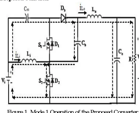
A. Mode 1 Operation of the Proposed Converter
Figure 1. Mode 1 Operation of the Proposed Converter
Figure 1 shows the modes 1 operation of the proposed converter. . The negative pulse is given to the switch S1 and
positive pulse is given to the switchS2 i.e., the switch S1 is turned off and S2 is turned on. In this mode of operation, the negative terminal of Cb is pulled to the ground, and hence, Db is forward-biased and turned on. From this, the
following equations are obtained.
⎩ ⎪ ⎪ ⎪ ⎪ ⎪ ⎨ ⎪ ⎪ ⎪ ⎪ ⎪ ⎧
dt dL L =
VLi i i
o C L
o dt =V -V
d L
m o
L o L o o
R V -i = dt dV C
o
o b m
L C C
m =i -i
dt dV C
(1)
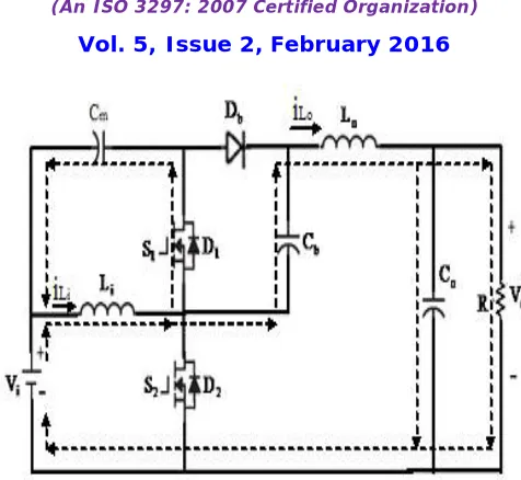
B. Mode 2 Operation of the Proposed Converter
Figure 2 shows the mode 2 operation of the proposed converter. The positive pulse is given to switch S1 i.e., the
switch S1 is turned ON. The negative pulse is given to switchS2 i.e., the switch S2 is turned OFF, and hence, Db is
Figure 2. Mode 2 Operation of the Proposed Converter
⎩ ⎪ ⎪ ⎪ ⎪ ⎨ ⎪ ⎪ ⎪ ⎪ ⎧
m i
C i L
i =V -V
dt di L
o C L
o =2V -V
dt d
L o m
L o L o o
R V -i = dt dV C
o
o i m
L L C
m =i -i
dt dV C
(2)
III.MATHEMATICAL MODELLING
The mathematical modelling of the converter with its transfer function are obtained from the following steps, a) The state variables are selected
b) Depending upon the modes, split the circuit and the substate model is obtained for each modes
c) Average large signal model is obtained
d) Steady state model
e) Small signal model
f)Transfer function
A. Selection of State Variables
The state variables are chosen to reflect the energy accumulation. In power electronic converters, it is considered as the current passing through the inductor, voltage across the capacitor and the combination of both. Here the state variables for both the KY boost converter and modified KY boost converter are mentioned. They are,
Input inductor current,
i
L i
Output inductor current,
o
L
i
Voltage across the capacitor Cm,m
C V
Voltage across the output capacitor,
V
oB. Substate Model for Both Modes
Bu + Ax = . x Du + Cx = y (3) Where,
A = State matrix which holds the property of the system. B = Input matrix which is the gain related to scaling the input. C = Scaling matrix.
D = Feedforward matrix. y = Controlled variable.
From Equation 1, the substate model for mode1 is given by,
dt d ⎣ ⎢ ⎢ ⎢ ⎢ ⎡ cm o o L i L v v i i ⎦ ⎥ ⎥ ⎥ ⎥ ⎤ = ⎣ ⎢ ⎢ ⎢ ⎢ ⎢ ⎢ ⎡ 0 0 C 1 -0 0 RC 1 -C 1 0 L 1 L 1 -0 0 0 0 0 0 m o o o o ⎦ ⎥ ⎥ ⎥ ⎥ ⎥ ⎥ ⎤ ⎣ ⎢ ⎢ ⎢ ⎢ ⎡ cm o o L i L v v i i ⎦ ⎥ ⎥ ⎥ ⎥ ⎤ + ⎣ ⎢ ⎢ ⎢ ⎢ ⎡ 0 0 0 L 1 i ⎦ ⎥ ⎥ ⎥ ⎥ ⎤ i V + ⎣ ⎢ ⎢ ⎢ ⎢ ⎢ ⎡ m C 1 0 0 0 ⎦ ⎥ ⎥ ⎥ ⎥ ⎥ ⎤ b C
i (4)
From Equation 2, the substate model for mode 2 is written as,
dt d ⎣ ⎢ ⎢ ⎢ ⎢ ⎡ cm o o L i L v v i i ⎦ ⎥ ⎥ ⎥ ⎥ ⎤ = ⎣ ⎢ ⎢ ⎢ ⎢ ⎢ ⎢ ⎢ ⎢ ⎡ 0 0 C 1 -C 1 0 RC 1 -C 1 0 L 2 L 1 -0 0 L 1 -0 0 0 m m o o o o i ⎦ ⎥ ⎥ ⎥ ⎥ ⎥ ⎥ ⎥ ⎥ ⎤ ⎣ ⎢ ⎢ ⎢ ⎢ ⎡ cm o o L i L v v i i ⎦ ⎥ ⎥ ⎥ ⎥ ⎤ + ⎣ ⎢ ⎢ ⎢ ⎢ ⎡ 0 0 0 L 1 i ⎦ ⎥ ⎥ ⎥ ⎥ ⎤ i
V (5)
C. Average Large Signal Model
These models replicate an average behaviour of the system state. It is the combination of both the modes
) d -1 ( A + d A =
A 1 2
) d -1 ( B + d B =
B 1 2
(6)
From the above equations, both the modes are combined together to get the large signal model.
D. Steady State Model
It is obtained in the equilibrium state. By zeroing the derivatives, one can obtain the steady state input-output characteristics (the locus of the systems equilibrium point). That isx0,dD,vo Vo, iLi ILi, iLo ILo,
m
m C
C V
v . Then the Equation 7 becomes
⎣ ⎢ ⎢ ⎢ ⎢ ⎢ ⎡
0
0
0
0
⎦ ⎥ ⎥ ⎥ ⎥ ⎥ ⎤
=
⎣ ⎢ ⎢ ⎢ ⎢ ⎢ ⎢ ⎢ ⎢ ⎡
0 0 C
) D -2 ( -C
D -1
0 RC
1 -C
1 0
L D -2 L
1 -0 0
L ) D -1 ( -0 0 0
m m
o o
o o
i
⎦ ⎥ ⎥ ⎥ ⎥ ⎥ ⎥ ⎥ ⎥ ⎤
⎣ ⎢ ⎢ ⎢ ⎢ ⎢ ⎡
cm o L L
V
V
I
I
o i
⎦ ⎥ ⎥ ⎥ ⎥ ⎥ ⎤
+
⎣ ⎢ ⎢ ⎢ ⎢ ⎢ ⎡
0 0 0 L 1
i
⎦ ⎥ ⎥ ⎥ ⎥ ⎥ ⎤
i
V (8)
out
V = 0 0 1 0
⎣ ⎢ ⎢ ⎢ ⎢ ⎢ ⎡
cm o L L
v
v
i
i
o i
⎦ ⎥ ⎥ ⎥ ⎥ ⎥ ⎤
(9)
In general, to find the input to output ratio in the steady state, Equation 10 can be used.
B CA -= V
V -1
i o
(10)
D -1
D -2 = V V
i o
(11)
The Equation 11 gives the resultant input to output ratio of the converter system in the steady state.
E. Small Signal Modelling
The converter dynamic behaviour is nonlinear with few exceptions. Sometimes, in order to perform a model analysis or to build linear control laws, it is necessary to develop linear models around a certain operating point. To this, the first order Taylor series expansion is used. These linearized models are valid only for slight variation around the operating point. This is why they are called small signal model or tangent linear models.
Conversely the initial models valid on the entire definition range are called large signal models. If the large signal model is linear, then it is identical to small signal model.
Small signal model is obtained by substituting in the average large signal model for every variable in steady state part, which is adding a small signal variation about the steady state or equilibrium point.
The state variables of the converter becomesd=D+dˆ,iLo =ILo +iˆLo , iLi =ILi+iˆLi, vCm =VCm+vˆCm, vo =Vo+vˆo
i i i =V +vˆ
dt
d
⎣ ⎢ ⎢ ⎢ ⎢ ⎢ ⎢ ⎡ m m o o i i C C o o L L L Lv
ˆ
+
V
v
ˆ
+
V
iˆ
+
I
iˆ
+
I
⎦ ⎥ ⎥ ⎥ ⎥ ⎥ ⎥ ⎤ = ⎣ ⎢ ⎢ ⎢ ⎢ ⎢ ⎢ ⎢ ⎢ ⎢ ⎢ ⎡ 0 0 C ) d ˆ -D -2 ( -C dˆ -D -1 0 RC 1 -C 1 0 L dˆ -D -2 L 1 -0 0 L ) d ˆ -D -1 ( -0 0 0 m m o o o o i ⎦ ⎥ ⎥ ⎥ ⎥ ⎥ ⎥ ⎥ ⎥ ⎥ ⎥ ⎤ ⎣ ⎢ ⎢ ⎢ ⎢ ⎢ ⎢ ⎡ m m o o i i C C o o L L L Lv
ˆ
+
V
v
ˆ
+
V
iˆ
+
I
iˆ
+
I
⎦ ⎥ ⎥ ⎥ ⎥ ⎥ ⎥ ⎤ + ⎣ ⎢ ⎢ ⎢ ⎢ ⎢ ⎡ 0 0 0 L 1 i ⎦ ⎥ ⎥ ⎥ ⎥ ⎥ ⎤ i i+vˆ V(12)
Equation 12 is a combination of both the steady state and the small signal model, the derivatives of the steady state part are eliminated i.e., zero. Then the small signal model obtained is shown in Equation 13.
dt d ⎣ ⎢ ⎢ ⎢ ⎢ ⎢ ⎢ ⎡ m o i C o L L
v
ˆ
v
ˆ
iˆ
iˆ
⎦ ⎥ ⎥ ⎥ ⎥ ⎥ ⎥ ⎤ = ⎣ ⎢ ⎢ ⎢ ⎢ ⎢ ⎢ ⎢ ⎢ ⎢ ⎡ 0 0 C ) D -2 ( -C D -1 0 RC 1 -C 1 0 L D -2 L 1 -0 0 L ) D -1 ( -0 0 0 m m o o o o i ⎦ ⎥ ⎥ ⎥ ⎥ ⎥ ⎥ ⎥ ⎥ ⎥ ⎤ ⎣ ⎢ ⎢ ⎢ ⎢ ⎢ ⎢ ⎡ m o i C o L Lv
ˆ
v
ˆ
iˆ
iˆ
⎦ ⎥ ⎥ ⎥ ⎥ ⎥ ⎥ ⎤ + ⎣ ⎢ ⎢ ⎢ ⎢ ⎢ ⎢ ⎢ ⎢ ⎡ 0 C I + C I -0 0 0 L V -L 1 L V m L m L o C i i C o i m m ⎦ ⎥ ⎥ ⎥ ⎥ ⎥ ⎥ ⎥ ⎥ ⎤ i vˆdˆ (13)
F. Transfer Function
From the small signal model, the transfer function can be obtained by using the Equation 14.
2 1 -i o B ) A -SI ( C = vˆ vˆ (14)
The input to the output voltage transfer function can be obtained as given in Equation 15,
o 1 2 2 3 3 4 4 i o a + s a + s a + s a + s a R ) D -1 )( D -2 ( = vˆ vˆ (15) Where, m o o i
4=RLL C C
a
m o i
3 =LL C
a o o o i m i o o i o o i 2
2 =D (L +L )C -2D(2L +L )C +LC +4LC +L C
a o i o i o i 2
1 =D (L +L )-D(4L +4L )+4L +4L
a
2 o =R(1-D) a
If the duty cycle is taken as the input function, then the control to output transfer function is obtained as given in Equation 16. o 1 2 2 3 3 4 4 o 1 2 2 o a + s a + s a + s a + s a b + s b + s b = dˆ vˆ (16) Where, R C L V -=
R )L I -D)(I --(2 =
b1 L L i
o i
R V D 2 + R 5DV -R V 3 =
b m m Cm
2 C
C o
IV. EXPERIMENTAL VALIDATION
In general PI controller has the ability to reject disturbances and can stabilize the process. A PI controller provides proficient output voltage regulation and reduced steady state error for both the converters.
The dc output voltage is sensed and compared with reference output voltage, which gives the error signal. This error signal is processed by the PI controller to keep the output voltage constant and reduce the steady state error. Here, the PI controller output sets the control signal for the converters. The PI controller parameters for the converters are given as trial and error.
By incorporating the transfer function in the PI controller, the proportional and the integral values are auto tuned and are obtained. With that tuned parameter values, the improved settling time and peak overshoot are obtained.
Figure3 Output Waveform of the Converter with PI Controller
Figure 3 shows the output voltage waveform of the converter with the settling time of 0.012s and the peak overshoot is 3V.
V. CONCLUSION
The state space averaging method is used to extend the analytical description of the proposed converter. Thus the linear transfer function for the proposed converter is derived. With this linearised transfer function, the closed loop performance of the proposed converter is done using the PI controller and so the fast settling of the converter is achieved.
As a future scope, the PI controller method is replaced by the soft computing techniques to improve the performance of the converter. With this the settling time and the peak overshoot of the converter is further improved.
REFERENCES
[1] Davoudi Ali, Juri Jatskevich, and Tom De Rybel, “Numerical state-space average-value modeling of PWM DC-DC converters operating in DCM and CCM”, IEEE Transactions on Power Electronics, Vol.21, No.4, pp. 1003-1012, 2006.
[2] Fang Lin Luo and Hong Ye, “Positive Output Super-Lift Converters”, IEEE Transaction on Power Electronics, Vol. 18, No. 1, pp. 105-113, 2003.
[3] Fang Lin Luo and Hong Ye., “Positive Output Multiple-Lift Push–Pull Switched-Capacitor Luo-Converters”, IEEE Transaction on Industrial Electronics, Vol. 51, No. 3, pp. 594-602, 2004.
[6] Hwu K. I. and Yau Y. T., “Voltage-Boosting Converter Based on Charge Pump and Coupling Inductor With Passive Voltage Clamping”, IEEE Transaction on Industrial Electronics, Vol. 57, No. 5, pp. 1719-1727, 2010.
[7] Hwu K. I. and Jiang W. Z., “Voltage Gain Enhancement for a Step-Up Converter Constructed by KY and Buck-Boost Converters”, IEEE Transaction on Industrial Electronics, Vol. 61, No. 4, pp. 1758-1768, 2014.
[8] Kuo-Ching Tseng, Chi-Chih Huang, Wei-Yuan Shih., “A High Step-Up Converter With a Voltage Multiplier Module for a Photovoltaic System”, IEEE Transaction on Power Electronics, Vol. 28, No. 6, pp. 3047-3057, 2013.
[9] Lai C. M. Pan C. T. and Cheng M. C, “High-efficiency Modular High Step-up Interleaved Boost Converter for DC-microgrid Applications”, IEEE Transaction on Industrial Electronics, Vol. 48, No. 1, pp. 161–171, 2012.
[10]Lung-Sheng Yang and Tsorng-Juu Liang, “Analysis and Implementation of a Novel Bidirectional DC–DC Converter”, IEEE Transaction Industrial Electronics, Vol. 59, No. 1, pp 422-434, 2012.
[11]Mattavelli, Paolo, Leopoldo Rossetto, and Giorgio Spiazzi, “General-purpose fuzzy controller for dc/dc converters”, IEEE Transaction on Power Electronics, Vol. 12, No. 1, pp.79-86, 1997.
[12]Pan C. T. and Lai C. M., “A High-Efficiency High Step-up Converter with Low Switch Voltage Stress for Fuel-cell System Applications”, IEEE Transaction Industrial Electronics, Vol. 57, No. 6, pp. 1998–2006, 2010.
[13]Perry, Alexander G, Guang Feng , Yan-Fei Liu , Sen, P.C., “A design method for PI-like fuzzy logic controllers for DC–DC converter”, IEEE Transactions on Industrial Electronics, Vol 54, No. 5, pp. 2688-2696, 2007.
[14]Priewasser Robert, Matteo Agostinelli and Christoph Unterrieder, “Modeling, control, and implementation of DC–DC converters for variable frequency operation”, IEEE Transactions on Power Electronics, Vol. 29, No.1, pp 287-301, 2014.
[15]Samosir, Ahmad Saudi, and Abdul Halim Mohd Yatim., “Dynamic evolution control for synchronous buck DC–DC converter: Theory, model and simulation”, Simulation Modelling Practice and Theory, Vol. 18, No.5, pp. 663-676, 2010.