Determination of Best Forecasting Method for Certain Types of Investment Methods in the Philippines

(1)

ISSN 2286-4822 www.euacademic.org

Impact Factor: 3.4546 (UIF) DRJI Value: 5.9 (B+)

Determination of Best Forecasting Method for

Certain Types of Investment Methods in the

Philippines

FRANCES ANNE A. CASTILLO

Philippine Statistics Authority

BRYAN S. BEATO

Lakewood College of Alabang

Abstract:

Most people are attaining financial security as they tend to save and invest money for a long period of time, thus, welcoming the idea of investment. A study was done to identify trends in the investment industry in the Philippines, to identify what investment type could yield optimum rate at maturity, and to forecast each investment method at three-year lead time. Investment methods include Treasury bills at 91, 182 and 364-day maturity, time deposits with less or more than one year maturity, savings deposits, and dividend yield ratio from stocks. Time series analysis was done on each variable. However, some assumptions were violated, thus, must only use the identified time series models with caution. Forecasting methods such as growth rate, trend model, and exponential smoothing were then introduced. It was found out that the growth rate and exponential smoothing has obtained the least mean absolute percentage errors (MAPE) from the forecasts. Also, comparison of yield interest rates at December 2018 was done, with the highest from the Treasury bill at 364-day maturity, however, its MAPE was highest among the said methods. Thus, it may be up to the consumer what to choose with the different methods given the said forecasts.

(2)

INTRODUCTION

One of the prime concerns of human being has always been avoidance of risks that threatened his existence and look forward for security. For the past years, investment managers and researchers have taken a revived interest on how to secure finances of every individual. The progress in the conceptualization of investment management models nowadays has occur simultaneously with much of this interest.

Most people are attaining financial security as they tend to save and invest money for a long period of time. The typical thinking of most people is, if you need money, you need to work. But is that collection of money going to be satisfying if you don’t have time to enjoy it? You can’t have a clone of yours to work every time for you so the expansion of money leads to an extension of your working hours. Investment is to make your money work for you, maximizing your potential earnings.

On an article entitled Investing 101 by a Wall Street

survivor, in investing, don’t look at how much the price of an investment went up or down in dollars and cents or “points” – look at its percentage gained or lost. The easiest way to understand how investments are changing in value daily, weekly, monthly or yearly is through percentages. Google (GOOG) went up $5 today and your General Electric (GE) stock went up 50 cents – which performed better for you? That might be a 1% return for GOOG but a 3% return for GE! Further, if the DJIA went up 500 points today for a 5% gain, why did your GOOG and GE underperform the market? Pay attention to the percentage changes in all of your assets and compare them to common market benchmarks. [8]

1.1 Objective of the Study

(3)

to: 1) to identify current trends in the investment industry through analyzing trends from each investment type; 2) to identify what investment type could possibly yield optimum rate in a certain period; and, 3) to identify the best forecasting method for each investment type.

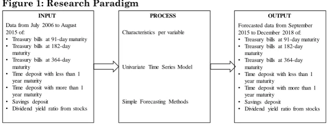
Figure 1: Research Paradigm

1.2 Statement of the Problem

This research aims to determine the interest rates yields from different investment types. It is of question which type of investing method may be best relied on when it comes to their interest rates. Given that the investment industry may also be a market with full of opportunities, it is of interest by the possible investors – both commercially and of personal reasons – to know the different investing methods in different statistical perspectives. In particular, the research aims to answer the following questions:

1. What are the characteristics of the following at present?

a. Treasury bills at 91-day maturity

b. Treasury bills at 182-day maturity

c. Treasury bills at 364-day maturity

d. Time deposit with less than 1 year maturity

e. Time deposit with more than 1 year maturity

f. Savings deposit

g. Dividend yield ratio from stocks

2. What are the forecasted interest rates of the following in

three-year time? Data from July 2006 to August

2015 of:

• Treasury bills at 91-day maturity

• Time deposit with less than 1 year maturity

• Time deposit with more than 1 year maturity

• Savings deposit

• Dividend yield ratio from stocks

Characteristics per variable

Univariate Time Series Model

Simple Forecasting Methods

Forecasted data from September 2015 to December 2018 of:

• Time deposit with less than 1 year maturity

• Time deposit with more than 1 year maturity

• Savings deposit

• Dividend yield ratio from stocks

(4)

a. Treasury bills at 91-day maturity

b. Treasury bills at 182-day maturity

c. Treasury bills at 364-day maturity

d. Time deposit with less than 1 year maturity

e. Time deposit with more than 1 year maturity

f. Savings deposit

g. Dividend yield ratio from stocks

3. Which forecasting method was used for generating

forecasts with least mean absolute percentage error?

1.3 Scope and Limitation

This study was limited by acknowledging that no attempt was made to test all of the investment types that are used to project the interest rates and return of investments. The study also limited to three (3) years interest rates obtained from the Bangko Sentral ng Pilipinas and the Philippine Stocks Exchange showing the interest rates starting from July 2006, until December 2015.

The investment types used in this study are limited to Time Deposits with maturity dates of less or greater than one year, Treasury bills with maturity dates at 91 days, 182 days and 364 days, Savings Deposits and Dividend Yield Ratio in Stocks.

REVIEW OF RELATED LITERATURE

This review of literature focuses mainly on three areas: (a) a historical review, (b) empirical findings from previous research on interest rates as determining factor in investment (i.e. GDP, Inflation), and (c) a summary of past research findings.

2.1 Historical Context

(5)

According to Sidney Homer and Richard Sylla [2] (2005), “Interest rate was used during historical era of Mesopotamia, Sumer, Babylonia and Assyria. The code of Hamurabi regulated the terms of ownership of land, the employment of agricultural labor, civil obligations as well as the commercial transactions. Absolute accounts had to be kept and negligence was penalized. From early times, down to the time of the Persian Empire, a span of thousands of years, the legislation on credit was noticeably stable. Loans without interest of consumable commodities were anticipated and they could, but need not, provide a penalty for repayment. Such penalty rates are common throughout history and must be sharply recognized from contract rates of interest. Seventeenth-century European finance was a study in contrasts. This era was often classified as “modern”. The legal rate of interest in England was as follows: 1571-1624 (10%), 1624-1651 (8%); 1651-1714 (6%). In Holland, short term deposits (1659-1700) has interest rate ranges from 3%-4%.” Furthermore, three economic events also affect the interest rates during the nineteenth century: a) organization of Federal Reserve System (1914-1917), b) the great depression of 1929-1939, c) the great inflation that started 1965. The steadiness of U.S. economic growth since 1990, even since the recession of 1981-1982, was by no means matched the behavior of interest rates. Bond yields of 15-16% became yields of 5-6%. Interest rates in the early 2000s were the lowest in four decades.

Interest rates changes as time changes. Nowadays, interest rates vary from country to country, currency to currency, as well as bank to bank. Many emerging markets are too new and too rapidly changing to have much of a continuous interest rate history.

(6)

According to Barry Bosworth (2014), the dominant influence of global factors suggests that interest rate projections should not incorporate any strong relationship to other economic trends in the domestic economy, such as those associated with the aging of the population, since they are likely to be overwhelmed by the global developments. They also stated the relationship of interest rates in different economic indicators as not a determining factor in the movements in inflation, the real GDP, aging of the population, exchange rate, money supply and NBU discount rate. [1]

The same result stated by Thomas Sargent (1976), in a study trying to show the relationship between Interest rate and Expected inflation. The article asserts the independence of the real rate of interest with respect to movements in inflation. [5]

Volodymyr Kosse (2002) conducted a study on the relationship between interest rates and other indicators in the economy in Ukraine, showed that despite theoretical importance of bank lending and commercial interest rate as its price for output growth, Ukrainian banking system does not influence real sector of economy as much as many economists and politicians would like. Volodymyr Kosse also found out that pairwise relationship between interest rates and inflation, exchange rate, money supply, real GDP and NBU discount rate. [3]

On the other hand, several researchers found out interest rate as a determining factor in investment. Different from the traditional theory, some scholars hypothesized that there was a positive correlation between investment and interest rate.

According to Wuhan, Li Suyuan, Adnan Khurshid (2015), in a study conducted in Jiangsu, China, the rate and investment have a positive relationship. Reducing the rate will promote investment in Jiangsu. [7]

(7)

leveraged by variable mortgage rates, this variability needs to be regulated (Muthaura, 2010). [4] This was also a finding in the research conducted by Kingsley Uche Sunday in Nigeria, interest rates have a positive significant impact on aggregate savings in Nigeria. This was confirmed by a positive interest rate coefficient. [6]

METHODOLOGY

3.1 Data

The data used were from the interactive database of the Bangko Sentral ng Pilipinas. These data were chronologically arranged, so that the data will be of time series. Variables gathered include weighted average interest rates on treasury bills at 91 days, treasury bills at 182 days, treasury bills at 364 days, time deposit in less than a year, time deposit in more than a year, savings deposits, and special deposits. These were measured monthly from the January 2000 to August 2015. At least fifty data points were used to ensure the accuracy of the forecast estimates using the models obtained.

3.2 Characteristics of Data Series

(8)

3.3 Time Series Analysis

Time series models were constructed to come up with possible forecasting models. These models underwent diagnostic checking, namely white noise test, Jarque-Bera normality test, Portmanteau lack-of-fit test, and ARCH LM test.

White noise test determines the series has a mean of 0 and constant variance. This test assumes that the distribution of the series is normal, independent, and uncorrelated.

The Jarque-Bera normality test aims to determine whether the residuals follow a normal distribution. The formula is as follows:

[ ( ) ]

wherein S and K are as follows:

∑ ( )

( ∑( ) )

and ∑ ( )

( ∑ ( ) )

.

Portmanteau lack-of-fit test determines whether there is no autocorrelation among the residuals of the series. The formula is as follows:

( ) ∑( ) _̂

wherein K is the maximum lag length ( ), n is the number of

observations, and ̂ is the sACF at lag k.

Lastly, ARCH LM test determines whether the residuals of the series have a constant variance or not. The formula is as follows:

(9)

3.4 Forecasting

The individual model per time series variable was used to forecast future values based on available data. Also, forecasting methods such as growth rate model, trend modelling, and double exponential smoothing methods were used for comparison of forecast values.

The formula for the growth rate is as follows:

and the forecast model is as follows:

(

) .

Trend models were obtained by graphing the time series data, then obtained a precise trend model that explained the behavior of the said series.

Double exponential smoothing, on the other hand, has the forecast formula as follows:

where the MEAN and TREND are the “intercept” and “slope”, respectively, of the forecast equation and computed as follows:

( )( )

( ) ( ) ,

while L is the forecast horizon from time t.

Initial run through data was done for forecast from September 2015 to December 2018. Data used was from 2006 to 2015. Mean absolute percentage error (MAPE) was used for assessment of the accuracy of the forecast with respect to the actual data. The formula is as follows:

(10)

where , yt denotes the actual value of

interest at time t, while ft denotes the forecast for the variable

of interest time t.

RESULTS AND DISCUSSION

4.1Characteristics of Time Series

The characteristics of the data series of each variable were checked in terms of its trend, cycle, seasonality, and irregularity.

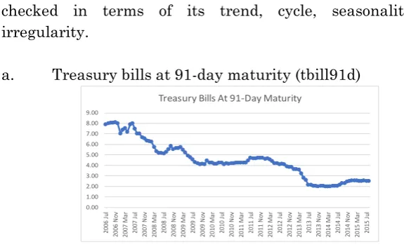
a. Treasury bills at 91-day maturity (tbill91d)

Figure 1 shows the graph of interest rates of Treasury bills at 91-day maturity. The data series has a downward trend, has no cycle, no seasonality, and no significant irregularity.

b. Treasury bills at 182-day maturity (tbill182d)

Table 3. Mean Absolute Percentage Errors of the Variables by Forecasting Methods.Figure 1. Graph of interest rates of Treasury bills at 91-day maturity.

0.00 1.00 2.00 3.00 4.00 5.00 6.00 7.00 8.00 9.00 20 06 J ul 20 06 N ov 20 07 M ar 20 07 J ul 20 07 N ov 20 08 M ar 20 08 J ul 20 08 N ov 20 09 M ar 20 09 J ul 20 09 N ov 20 10 M ar 20 10 J ul 20 10 N ov 20 11 M ar 20 11 J ul 20 11 N ov 20 12 M ar 20 12 J ul 20 12 N ov 20 13 M ar 20 13 J ul 20 13 N ov 20 14 M ar 20 14 J ul 20 14 N ov 20 15 M ar 20 15 J ul

Treasury Bills At 91-Day Maturity

Figure 2. Graph of interest rates of Treasury bills at 182-day maturity.

0.00 1.00 2.00 3.00 4.00 5.00 6.00 7.00 8.00 9.00 20 06 J ul 20 06 N ov 20 07 M ar 20 07 J ul 20 07 N ov 20 08 M ar 20 08 J ul 20 08 N ov 20 09 M ar 20 09 J ul 20 09 N ov 20 10 M ar 20 10 J ul 20 10 N ov 20 11 M ar 20 11 J ul 20 11 N ov 20 12 M ar 20 12 J ul 20 12 N ov 20 13 M ar 20 13 J ul 20 13 N ov 20 14 M ar 20 14 J ul 20 14 N ov 20 15 M ar 20 15 J ul

(11)

Figure 2 shows the graph of interest rates of Treasury bills at 182-day maturity. The data series has a downward trend, has no cycle, no seasonality, and no significant irregularity.

c. Treasury bills at 364-day maturity (tbill364d)

Figure 3 shows the graph of interest rates of Treasury bills at 364-day maturity. The data series has a downward trend, has no cycle, and no seasonality. However, sudden decreases were observed during January to February 2009, and October to December 2010.

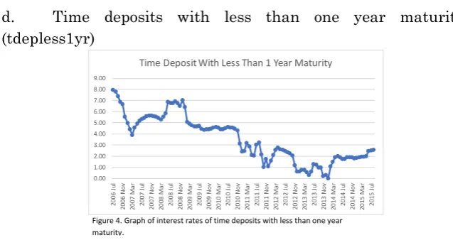
d. Time deposits with less than one year maturity

(tdepless1yr)

Figure 4 shows the graph of interest rates of time deposits with less than one maturity. The data series has generally a downward trend, has no cycle, and no seasonality. Sudden

0.00 1.00 2.00 3.00 4.00 5.00 6.00 7.00 20 06 J ul 20 06 N ov 20 07 M ar 20 07 J ul 20 07 N ov 20 08 M ar 20 08 J ul 20 08 N ov 20 09 M ar 20 09 J ul 20 09 N ov 20 10 M ar 20 10 J ul 20 10 N ov 20 11 M ar 20 11 J ul 20 11 N ov 20 12 M ar 20 12 J ul 20 12 N ov 20 13 M ar 20 13 J ul 20 13 N ov 20 14 M ar 20 14 J ul 20 14 N ov 20 15 M ar 20 15 J ul

Figure 3. Graph of interest rates of Treasury bills at 364-day maturity.

Figure 4. Graph of interest rates of time deposits with less than one year maturity. 0.00 1.00 2.00 3.00 4.00 5.00 6.00 7.00 8.00 9.00 2 0 0 6 J u l 2 0 0 6 N o v 2 0 0 7 M a r 2 0 0 7 J u l 2 0 0 7 N o v 2 0 0 8 M a r 2 0 0 8 J u l 2 0 0 8 N o v 2 0 0 9 M a r 2 0 0 9 J u l 2 0 0 9 N o v 2 0 1 0 M a r 2 0 1 0 J u l 2 0 1 0 N o v 2 0 1 1 M a r 2 0 1 1 J u l 2 0 1 1 N o v 2 0 1 2 M a r 2 0 1 2 J u l 2 0 1 2 N o v 2 0 1 3 M a r 2 0 1 3 J u l 2 0 1 3 N o v 2 0 1 4 M a r 2 0 1 4 J u l 2 0 1 4 N o v 2 0 1 5 M a r 2 0 1 5 J u l

(12)

increase was observed during April to June 2008, but has subsided starting December of the same year. Also, ups and downs were experienced during November 2010 to April 2012, and October 2012 to April 2014.

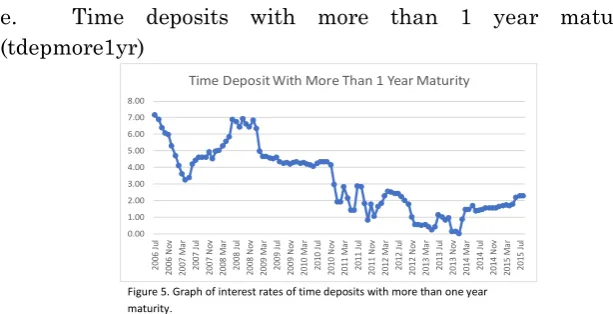
e. Time deposits with more than 1 year maturity

(tdepmore1yr)

Figure 5 shows the graph of interest rates of time deposits with more than one maturity. The data series has generally a downward trend, has no cycle, and no seasonality. Sudden decrease was observed from December 2008 to March 2009. Also, ups and downs were experienced starting November 2010, up to April 2012. Moreover, decreases were observed at the last quarter of 2012 and 2013, but has increased after the third quarter of 2013, and first quarter of 2014, respectively.

f. Savings deposits (savdep)

Figure 5. Graph of interest rates of time deposits with more than one year maturity. 0.00 1.00 2.00 3.00 4.00 5.00 6.00 7.00 8.00 20 06 J ul 20 06 N ov 20 07 M ar 20 07 J ul 20 07 N ov 20 08 M ar 20 08 J ul 20 08 N ov 20 09 M ar 20 09 J ul 20 09 N ov 20 10 M ar 20 10 J ul 20 10 N ov 20 11 M ar 20 11 J ul 20 11 N ov 20 12 M ar 20 12 J ul 20 12 N ov 20 13 M ar 20 13 J ul 20 13 N ov 20 14 M ar 20 14 J ul 20 14 N ov 20 15 M ar 20 15 J ul

Time Deposit With More Than 1 Year Maturity

Figure 6. Graph of interest rates of savings deposits.

(13)

Figure 6 shows the graph of interest rates of savings deposits. The data series has a downward trend, has no cycle, and no seasonality. Sudden decrease starting January 2009 was observed, and periodic decrease started during February 2013.

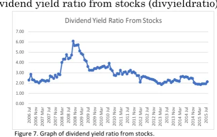
g. Dividend yield ratio from stocks (divyieldratio)

Figure 7 shows the graph of interest rates of savings deposits. The data series has generally monotonous flat trend, has no cycle, and no seasonality. Increases were observed during February 2008, and has subsided during August 2009.

4.2 Model Identification and Diagnostic Checking

After analyzing the trends of each variable, Augmented Dickey-Fuller test and evaluation of correlogram was done in order to identify corresponding time series models. Given the variables, two sets of models per identified: one from the original data series, and one from transformed data series. All variables have undergone data series transformation through natural logarithm.

Figure 7. Graph of dividend yield ratio from stocks.

0.00 1.00 2.00 3.00 4.00 5.00 6.00 7.00 2 0 0 6 J u l 2 0 0 6 N o v 2 0 0 7 M a r 2 0 0 7 J u l 2 0 0 7 N o v 2 0 0 8 M a r 2 0 0 8 J u l 2 0 0 8 N o v 2 0 0 9 M a r 2 0 0 9 J u l 2 0 0 9 N o v 2 0 1 0 M a r 2 0 1 0 J u l 2 0 1 0 N o v 2 0 1 1 M a r 2 0 1 1 J u l 2 0 1 1 N o v 2 0 1 2 M a r 2 0 1 2 J u l 2 0 1 2 N o v 2 0 1 3 M a r 2 0 1 3 J u l 2 0 1 3 N o v 2 0 1 4 M a r 2 0 1 4 J u l 2 0 1 4 N o v 2 0 1 5 M a r 2 0 1 5 J u l

(14)

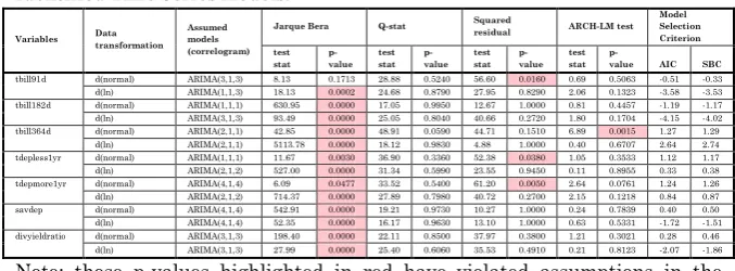
Table 1. Results of Different Model Diagnostics Checking Tests for the Identified Time Series Models.

Variables Data _{transformation} Assumed models (correlogram)

Jarque Bera Q-stat Squared _residual ARCH-LM test Model Selection Criterion test

stat p-value

test stat

p-value

test stat

p-value

test stat

p-value AIC SBC

tbill91d d(normal) ARIMA(3,1,3) 8.13 0.1713 28.88 0.5240 56.60 0.0160 0.69 0.5063 -0.51 -0.33 d(ln) ARIMA(1,1,3) 18.13 0.0002 24.68 0.8790 27.95 0.8290 2.06 0.1323 -3.58 -3.53 tbill182d d(normal) ARIMA(1,1,1) 630.95 0.0000 17.05 0.9950 12.67 1.0000 0.81 0.4457 -1.19 -1.17 d(ln) ARIMA(3,1,3) 93.49 0.0000 25.05 0.8040 40.66 0.2720 1.80 0.1704 -4.15 -4.02 tbill364d d(normal) ARIMA(2,1,1) 42.85 0.0000 48.91 0.0590 44.71 0.1510 6.89 0.0015 1.27 1.29 d(ln) ARIMA(2,1,1) 5113.78 0.0000 18.12 0.9830 4.88 1.0000 0.40 0.6707 2.64 2.74 tdepless1yr d(normal) ARIMA(1,1,1) 11.67 0.0030 36.90 0.3360 52.38 0.0380 1.05 0.3533 1.12 1.17 d(ln) ARIMA(2,1,2) 527.00 0.0000 31.34 0.5990 23.55 0.9450 0.11 0.8955 0.33 0.38 tdepmore1yr d(normal) ARIMA(4,1,4) 6.09 0.0477 33.52 0.5400 61.20 0.0050 2.64 0.0761 1.24 1.26 d(ln) ARIMA(2,1,2) 714.37 0.0000 27.89 0.7980 40.72 0.2700 2.15 0.1218 0.84 0.87 savdep d(normal) ARIMA(4,1,4) 542.91 0.0000 19.21 0.9730 10.27 1.0000 0.24 0.7839 0.40 0.50 d(ln) ARIMA(4,1,4) 52.35 0.0000 16.17 0.9630 13.10 1.0000 0.63 0.5331 -1.72 -1.51 divyieldratio d(normal) ARIMA(3,1,3) 198.40 0.0000 22.11 0.8500 37.97 0.3800 1.21 0.3021 0.28 0.46 d(ln) ARIMA(3,1,3) 27.99 0.0000 25.40 0.6060 35.53 0.4910 0.21 0.8123 -2.07 -1.86 Note: those p-values highlighted in red have violated assumptions in the model diagnostic checking on time series models.

Table 1 shows the results for the different kinds of test for the diagnostic checking for all the identified time series models. Given these results, this may mean that all the identified time series models may only be used with caution. These models may generate high root mean square error (RMSE) and mean absolute percentage error (MAPE).

For the Jarque-Bera test for normality, only one model has passed the criteria, which is the Treasury bill at 91-day maturity from normal data. All other generated models have violated the assumption on normality. For the Portmanteau Lack-of-Fit test or Q-stat, all models have passed the assumption on autocorrelation of the residuals. All have passed the criteria of p-value exceeding the set alpha of 0.05. Three models have violated the assumption of homogeneity of variance. These models were Treasury bill at 91-day maturity from normal data, time deposits with less than one year maturity from normal data, and time deposits with more than one year maturity from normal data. For the ARCH-LM test, only one model has failed the criteria, which is the Treasury bill at 364-day maturity from normal data. Other models have satisfied the assumption of constant error variance.

(15)

precise forecasts. Thus, models were created from other forecasting methods, such as growth rates, trend models, and exponential smoothing.

Table 2. Identifies Simple Forecasting Models from Variables.

Variables Growth Rate Trend Model

Exponential Smoothing tbill91d y = 0.0003x2 - 0.084x + _7.9087 Alpha _Beta 1.00 _0.00 tbill182d

y = 0.0003x2 - 0.0861x + 7.9357

Alpha 1.00 Beta 0.68 tbill364d y = 0.0002x2 - 0.0666x + _5.695 Alpha _Beta 1.00 _0.01 tdepless1y

r

y = 0.0003x2 - 0.0919x + 7.26

Alpha 1.00 Beta 0.01 tdepmore1

yr

y = 0.0002x2 - 0.0739x + 6.4599

Alpha 1.00 Beta 0.01 savdep y = -1E-04x2 - 0.0189x +

4.2205

Alpha 1.00 Beta 0.00 divyieldra

tio

y = -0.0005x2 + 0.0376x + 2.685

Alpha 0.94 Beta 0.00

Table 2 shows the identified simple forecasting models from the given variables. The growth rate was computed with the standard formula of proportion of change from its previous data. On the other hand, the identified trend models for each variable were taken from initial trends of the variables. Then, the exponential smoothing for each variable were based from Holt-Winter’s exponential smoothing. As can be observed, most of the alpha values were near to one, while the beta values were lower, or even zero.

4.3 Forecasting

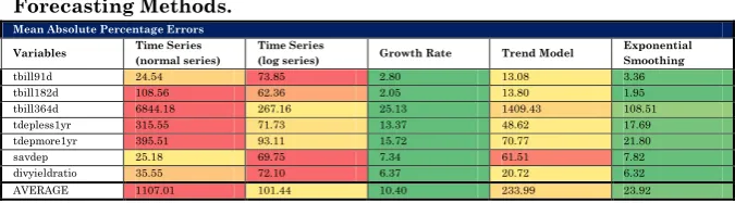
Table 3. Mean Absolute Percentage Errors of the Variables by Forecasting Methods.

Mean Absolute Percentage Errors

Variables Time Series _{(normal series)} Time Series _{(log series)} Growth Rate Trend Model Exponential _Smoothing

tbill91d 24.54 73.85 2.80 13.08 3.36

tbill182d 108.56 62.36 2.05 13.80 1.95

tbill364d 6844.18 267.16 25.13 1409.43 108.51

tdepless1yr 315.55 71.73 13.37 48.62 17.69

tdepmore1yr 395.51 93.11 15.72 70.77 21.80

savdep 25.18 69.75 7.34 61.51 7.82

divyieldratio 35.55 72.10 6.37 20.72 6.32

(16)

Table 3 shows the mean absolute percentage errors from different forecasting methods. On the average, the forecasting method with the least average mean absolute percentage errors (MAPE) from all of the treated variables was growth rate. On the other hand, the highest MAPE was the time series model created from the normal data series. Most variables had the growth rate with the least MAPE, while the Treasury bill at 364-day maturity and dividend yield ratio from stocks had the exponential smoothing with the least MAPE.

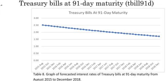
a. Treasury bills at 91-day maturity (tbill91d)

Table 8 shows the forecasted interest rates of Treasury bills at 91-day maturity from August 2015 to December 2018. As can be seen, the forecasts are observed to have a decreasing trend. The mean growth rate that was estimated from 2006 to 2015 data was -0.96%, thus explains the said trend. On December 2018, it is expected that the interest rate of Treasury bills at 91-day maturity will be 1.71%, with noted mean absolute percentage error of 2.80%.

Table 8. Graph of forecasted interest rates of Treasury bills at 91-day maturity from August 2015 to December 2018.

0.00 0.50 1.00 1.50 2.00 2.50 3.00

(17)

b. Treasury bills at 182-day maturity (tbill182d)

Table 9 shows the forecasted interest rates of Treasury bills at 182-day maturity from August 2015 to December 2018. As can be seen, the forecasts are observed to have a constant trend. Holt-Winter’s Double Exponential Smoothing was used to forecast the said series. On December 2018, it is expected that the interest rate of Treasury bills at 91-day maturity will be 2.50%, with noted mean absolute percentage error of 1.95%.

c. Treasury bills at 364-day maturity (tbill364d)

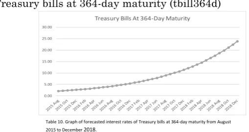
Table 10 shows the forecasted interest rates of Treasury bills at 364-day maturity from August 2015 to December 2018. It may be observed that the forecasted interest rates have an increasing trend. The mean growth rate estimated was 6.37%, thus explains the trend. The forecast for the interest rate of the Treasury bills at 364-day maturity is at 23.86%. However, it

1.80 1.90 2.00 2.10 2.20 2.30 2.40 2.50 2.60

0.00 5.00 10.00 15.00 20.00 25.00 30.00

(18)

may also be noted that the mean absolute percentage error is 25.13%, which may denote that the said forecast may be 25.13% off from the actual value.

d. Time deposits with less than one year maturity (tdepless1yr)

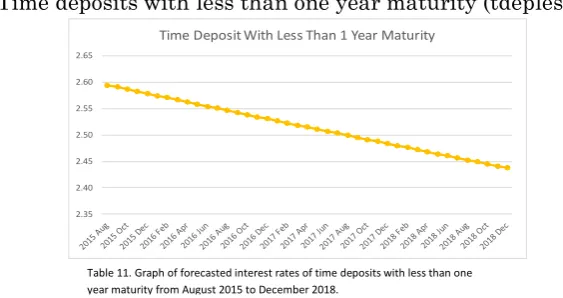
Table 11 shows the forecasted interest rates of time deposits with less than one year maturity from August 2015 to December 2018. It may be observed that the forecasted interest rates have a decreasing trend. The mean growth rate estimated was -0.16%, thus explains the trend. The forecast for the interest rate of the time deposits with less than one year maturity is at 2.44%, with mean absolute percentage error of 13.37%.

e. Time deposits with more than 1 year maturity

(tdepmore1yr)

Table 11. Graph of forecasted interest rates of time deposits with less than one year maturity from August 2015 to December 2018.

2.35 2.40 2.45 2.50 2.55 2.60 2.65

Time Deposit With Less Than 1 Year Maturity

Table 12. Graph of forecasted interest rates of time deposits with more than one year maturity from August 2015 to December 2018.

0.00 0.50 1.00 1.50 2.00 2.50 3.00

(19)

Table 12 shows the forecasted interest rates of time deposits with more than one year maturity from August 2015 to December 2018. As can be seen, the forecasts are observed to have an increasing trend. The mean growth rate that was estimated from 2006 to 2015 data was 0.54%, thus explains the said trend. On December 2018, it is expected that the interest rate of Treasury bills at 91-day maturity will be 2.78%, with noted mean absolute percentage error of 15.72%.

f. Savings deposits (savdep)

Table 13 shows the forecasted interest rates of savings deposits from August 2015 to December 2018. It may be observed that the forecasted interest rates have a decreasing trend. The mean growth rate estimated was -0.70%, thus explains the trend. The forecast for the interest rate of the time deposits with less than one year maturity is at 1.04%, with mean absolute percentage error of 7.34%.

g. Dividend yield ratio from stocks (divyieldratio)

Table 13. Graph of forecasted interest rates of savings deposits from August 2015 to December 2018.

0.00 0.20 0.40 0.60 0.80 1.00 1.20 1.40 1.60

Savings Deposit

Table 14. Graph of forecasted interest rates of dividend yield ratio from stocks from August 2015 to December 2018.

0.00 0.50 1.00 1.50 2.00 2.50 3.00

(20)

Table 14 shows the forecasted interest rates of dividend yield ratio from stocks from August 2015 to December 2018. As can be seen, the forecasts are observed to have an increasing trend. Holt-Winter’s Double Exponential Smoothing was used to forecast the said series. On December 2018, it is expected that the interest rate of Treasury bills at 91-day maturity will be 2.55%, with noted mean absolute percentage error of 6.32%.

CONCLUSION AND RECOMMENDATION

5.1 Conclusion

The time series models generated from the original and transformed data did not satisfy primary assumptions for a sound model. Thus, time series models generated may be used but with most caution, as these models may produce estimates with high forecast errors. Generation of models from different simple forecasting methods were done then.

Based on the mean absolute percentage errors (MAPE) from time series models, mean growth rates, trend models, and exponential smoothing, most of the investment methods had the least MAPE from the mean growth rates. Two methods (Treasury bills at 182-day maturity and dividend yield ratio from stocks) had the exponential smoothing with the least MAPE. It may be preferred to use these forecasting methods, but should still be tested for their MAPE.

(21)

5.2 Recommendation

It may be recommended that further conduct of study may include other various investment methods. In this way, other investment methods may be statistically tested and forecasted. Also, data earlier than July 2006 may be included as part of the data series, in order to fully account the earlier trends, possible cycle, seasonality, and irregularity available. This may help to give a further explanation to the resulting forecast data series.

REFERENCES

[1] Bosworth, B. (2014). Interest Rate and Economic Growth:

Are they related? Retrieved from:

http://crr.bc.edu/working-papers/interest-rates-and-economic-growth-are-they-related/

[2] Homer S., Sylla R. (2005). A History Of Interest Rates: 4th

edition. Retrieved from:

https://www.docdroid.net/n9ka/sidney-homer-richard-sylla-a-history-of-interest-rates.pdf.html#page=9

[3] Kosse V. (2002). Interest rate and theiry role in the economy

during the transition. The Problem of High Interest Rates, Case

of Ukraine. Retrieved from:

http://www.kse.org.ua/uploads/file/library/2002/Kosse_Volodym yr.pdf

[4] Muthaura, A. (2012). The Relationship between Interest rate

and Real Estate Investment. Retrieved from:

http://erepository.uonbi.ac.ke/bitstream/handle/11295/14367/M uthaura_The%20relationship%20between%20interest%20rates %20and%20real%20Estate%20investment%20in%20Kenya.pdf? sequence=4

[5] Sargent, T. (1985). Interest Rates and Expected Inflation: A

Selective Summary of Recent Research. In Explorations in

Economic Research, Volume 3, Number 3 (pp. 303-325).

Retrieved from: http://www.nber.org/chapters/c9082.pdf

[6] Sunday, K. (2012). The impact of Interest Rates on savings

(22)

http://www.unn.edu.ng/publications/files/images/SUNDAY,%20 KINGSLEY%20UCHE.pdf

[7] Wuhan, Li & Khurshid A. (2015). The effect of interest rate

on investment: Empirical evidence of Jiangsu Province, China.

Retrieved from:

http://www.jois.eu/files/JIS_Vol8_No1_Wuhan_Suyuan_Khursh id.pdf

[8] Investing 101. (n.d.) Retrieved from