P R O C E E D I N G S
Open Access
Novel tree-based method to generate markers
from rare variant data
Yuan Jiang, Jennifer S Brennan, Rose Calixte, Yunxiao He, Epiphanie Nyirabahizi, Heping Zhang
*From
Genetic Analysis Workshop 17
Boston, MA, USA. 13-16 October 2010
Abstract
Existing methods for analyzing rare variant data focus on collapsing a group of rare variants into a single common variant; collapsing is based on an intuitive function of the rare variant genotype information, such as an indicator function or a weighted sum. It is more natural, however, to take into account the single-nucleotide polymorphism (SNP) interactions informed directly by the data. We propose a novel tree-based method that automatically detects SNP interactions and generates candidate markers from the original pool of rare variants. In addition, we utilize the advantage of having 200 phenotype replications in the Genetic Analysis Workshop 17 data to assess the candidate markers by means of repeated logistic regressions. This new approach shows potential in the rare variant analysis. We correctly identify the association between geneFLT1and phenotype Affect, although there exist other false positives in our results. Our analyses are performed without knowledge of the underlying simulating model.
Background
Recent work supports the involvement of rare variants in complex disease etiology [1-3]; despite a low fre-quency of occurrence, rare variants may be functionally important and may account for a detectable increase in the relative risk of developing the outcome. Next-gen-eration sequencing has great potential for important applications in human genetics, including the detection of rare variants. Several methods have been proposed to handle rare variants in association analyses [4-7]. The aim of these methods is to construct a set of markers from the original single-nucleotide polymorphisms (SNPs), using predefined groups, such as genes or nearby genomic regions. These candidate markers are then considered in an association analysis.
For example, a key analytical tool is the collapsing method. Named for the collapsing of genotypes across variants, the collapsing method uses a rare variant indi-cator for each subject to describe the presence of rare variants in prespecified subsets of SNPs. Li and Leal [5]
extended the collapsing method to the framework of multiple-marker tests, and called their method the com-bined multivariate and collapsing (CMC) method. They proposed dividing the markers into subgroups according to specific criteria and then collapsing the genotypes within each group. Morris and Zeggini’s [7] collapsing method uses an indicator variable for the presence of the rare variants and a quantitative variable for the pro-portion of the variants that carry at least one copy of the minor allele. Madsen and Browning [6] developed a weighted-sum statistic as a groupwise association test for rare variants. Their method constructs markers by taking a weighted sum of the number of rare variants from a subset of SNPs. The weights depend on the mutation frequency in the unaffected individuals. Although these methods are intuitive and easy to imple-ment, they construct the markers without considering SNP interactions.
The goal of our paper is to develop an approach that constructs meaningful markers generated from the data. As in previous methods, we aim to define a single mar-ker for a set of SNPs. However, our framework focuses on detecting the interaction among these SNPs by fitting a phenotype association model. Interaction among a group of SNPs describes the situation in which the joint * Correspondence: [email protected]
Department of Epidemiology and Public Health, Yale School of Public Health, School of Medicine, Yale University, 60 College Street, PO Box 208034, New Haven, CT 06520-8034, USA
influence of this group on the response variable is not additive. Because most of the SNPs are rare, a regression model including explicit interactions is unaffordable and lacks power. Thus we use the recursive partitioning method to automatically search the interactions between the SNPs in an explicit way. Once interactions are detected among a group of SNPs, we can define a mar-ker specifically by these interactions.
Methods
Preprocessing
We assessed deviations from Hardy-Weinberg equili-brium (HWE) for common variants [8]. All SNPs with a minor allele frequency (MAF) greater than 0.05 that failed the HWE test (p < 0.0001) were excluded from further analysis.
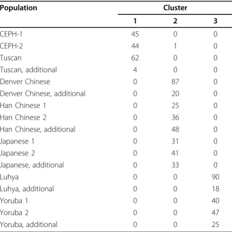
We conducted an analysis to identify population stra-tification using PLINK [9]. We then computed a similar-ity matrix based on the pairwise identsimilar-ity-by-state (IBS) distances. Next we performed a multidimensional scal-ing (MDS) analysis on the similarity matrix. Finally, we used the pam function (a modified, more robust con-struction of Kmeans) in the R package to perform a cluster analysis with the terminal cluster number set to 3.
Combining SNPs into markers using recursive partitioning
Statistical interaction describes the situation in which the simultaneous influence of a group of explanatory variables on the response variable is not additive. Recur-sive partitioning is a natural nonparametric approach to modeling interactions among a group of variables [10,11]. Ultimately, the recursive partitioning framework meaningfully groups the rare variants into what are essentially common variants. Depending on the format of a phenotype, a classification or regression tree can be applied. For the sake of clarity, we consider only the simplest case: a binary classification tree for a binary response.
We used the first replication of the phenotype in the Genetic Analysis Workshop 17 (GAW17) data to con-struct the classification tree. Here, Affected, denoted by Y, is the binary outcome (case or control, or 1 or 0) used as the response to construct the classification tree. A single binary classification tree can be grown for all SNPs within a shared gene. The tree grows as a result of recursively partitioning a node by a single SNP into two daughter nodes. Because we consider a SNP to be a three-level factor variable X, with levels 0, 1, and 2, the partitioning occurs whenX is partitioned as {0} and {1, 2} or as {0, 1} and {2}. Once a tree model is built, each terminal leaf node contains a set of observations, which are predicted as case subjects or control subjects (1 or 0). This terminal node takes on the value of the
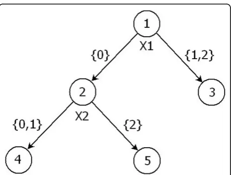
outcome majority of observations in that node. We illus-trate the construction of a marker using the example tree model in Figure 1.
Suppose that the example tree shown in Figure 1 is fitted using phenotype Yand a group of SNP variables X1,X2, X3, andX4. Let’s consider the case that X1 and X2 are used as the partitioning variables (thus X1, X2, X3, andX4are the searched SNPs andX1 andX2are the final SNPs used in the tree). Accordingly, the tree indi-cates an interaction between X1 and X2. Suppose that the leaf nodes 3 and 4 contain a majority of“control” subjects; these two leaf nodes are then also considered
“control” leaves. Similarly, if leaf node 5 contains a majority of “case” subjects, then node 5 is considered a
“case” leaf. The path to reach each of these three leaf nodes from the initial root is described by the tree’s three branches: {B1: X1 > 0}, {B2: X1 = 0 and X2 < 2}, {B3: X1 = 0 andX2 = 2}. Thus the branchesB1 andB2 have the same effect direction because they both result in a “control” prediction. B3, however, has the reverse effect direction because it results in a“case” prediction. Thus a bilevel marker can be constructed: one level of the marker represents B1andB2, and the other level of the marker representsB3. It is noteworthy that this bile-vel marker is exactly the same as the fitted value of Y for all of the subjects.
For the GAW17 data set, each SNP belongs to one and only one gene, thus providing a natural set of groups, each of which can generate a tree. Therefore each marker is defined using the fitted value of Y for
Figure 1Example tree.An example tree fitted using phenotypeY
and a group of SNP variablesX1,X2,X3, andX4.X1andX2are used
as the partitioning variables, yielding three leaf nodes.X1,X2,X3, and
X4are the searched SNPs, andX1andX2are the final SNPs used in
each gene, so long as the marker is not rare (our thresh-old was 1−0.992 = 0.0199). Many genes, however, had a very small number of SNPs (e.g., 1,226 genes had only 1 SNP and 440 genes had 2 SNPs). For these genes with few typed SNPs, a tree can still be built using the sparse SNPs. However, use of such SNPs in trees still generates markers that have rare minor alleles. This motivates the following two-step procedure to construct the markers on a chromosome:
Step 1. For each gene on the chromosome, build a
tree model for the phenotype Affected using the SNPs contained in that gene. Record a single marker for each gene if the minor allele of the marker is not rare.
Step 2.For all the remaining SNPs not considered in step 1, perform a clustering analysis to cluster nearby SNPs on the chromosome. If the minor allele of the marker is not rare, consider this marker in tree con-struction from each cluster of SNPs.
Evaluating the markers by repeated independent logistic regressions
We used only the first replication of the phenotype Affected to construct the markers; the remaining 199 phenotype replications were used to evaluate these mar-kers. To evaluate each marker, we fitted a logistic regression using Affected as the response variable against each marker, adjusted for sex, age, smoking sta-tus, and race (ethnicity) cluster covariates.
For each marker, there are 199p-values resulting from the 199 independent tests. To assess the relative impor-tance of each marker, we report the number of replica-tions in which the marker achieves significance using a Bonferroni correction (p< 0.05/570). As a comparison, we make use of a false discovery rate (FDR) control [12] and report again the number of significant replications.
Results and discussion
Of the 24,487 SNPs, 87.2% (n = 21,355) have MAF < 0.05, 74.0% (n= 18,131) have MAF < 0.01, and 38.5% (n = 9,433) have MAF < 0.001. Those MAFs that are less than 0.001 are all equal to 0.000717. Because we have 697 unrelated individuals, 9,433 SNPs have a single minor allele across the whole sample, indicating that the coded variables for these 9,433 SNPs are a vector with 696 0’s and a single 1. This is quite problematic from a statistical point of view. Both univariate and multivariate association analyses are drastically underpowered and will not directly work for these particularly sparse variables.
We conducted an analysis to identify population stra-tification and to produce a similarity matrix based on the pairwise IBS distances. We then used the similarity matrix to perform an MDS analysis. The plot of the first two MDS dimensions reveals a clear clustering structure
of three distinct groups. The three resulting clusters from the pam function in R almost identically match the population structure, and three homogeneous ethnic groups can be identified (Table 1).
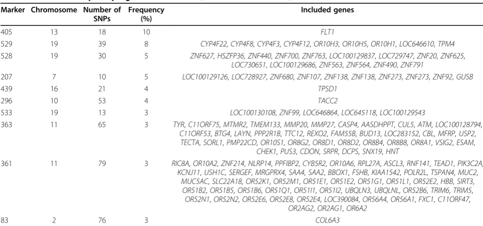
We identified 570 genome-wide markers after our two-step recursive partitioning method was carried out. Thus the final marker set is composed of markers from both the analysis considering SNPs in each gene sepa-rately and the analysis considering the combination of nearby SNPs in each cluster. Figure 2 provides two his-tograms of SNPs in the tree construction. The left-hand panel presents the number of SNPs that were searched by recursive partitioning. The right-hand panel presents the number of SNPs that were ultimately used in the tree when constructing each marker from a pool of SNPs (see the example tree in Figure 1). It is obvious that the number of searched SNPs must be greater than the number of finally used SNPs for each marker. It is noteworthy that most of the 570 generated markers consist of fewer than 30 SNPs, and the modest number of involved SNPs in each constructed marker simplifies the interpretation of the marker.
For each of the 570 constructed markers, we have 199 p-values from 199 replications. We report the number of replications in which the marker achieves the Bonfer-roni-corrected significance level (p< 0.05/570). Table 2 provides the 10 most frequently significant markers. The top marker, significant in 10 (out of 199) replicates, is derived from a tree that includes only the SNPs in the gene FLT1, which is a true signal [13]. This positive result demonstrates the potential of combining SNPs according to their interactions. The remaining nine
Table 1 Populations and corresponding clusters
Population Cluster
1 2 3
CEPH-1 45 0 0
CEPH-2 44 1 0
Tuscan 62 0 0
Tuscan, additional 4 0 0
Denver Chinese 0 87 0
Denver Chinese, additional 0 20 0
Han Chinese 1 0 25 0
Han Chinese 2 0 36 0
Han Chinese, additional 0 48 0
Japanese 1 0 31 0
Japanese 2 0 41 0
Japanese, additional 0 33 0
Luhya 0 0 90
Luhya, additional 0 0 18
Yoruba 1 0 0 40
Yoruba 2 0 0 47
Figure 2SNP numbers that were searched (left panel) and finally used (right panel) in the 570 markers.The left-hand panel indicates that there were relatively few cases with more than 100 searched SNPs; thus we omit these in the plot for a more clear comparison. The right-hand panel indicates the SNPs that were used to split the tree. Note that most of the 570 markers consist of fewer than 30 SNPs, which simplifies the interpretation of the generated markers.
Table 2 Ten most frequently significant markers (Bonferroni correction) Marker Chromosome Number of
SNPs
Frequency (%)
Included genes
405 13 18 10 FLT1
529 19 39 8 CYP4F22,CYP4F8,CYP4F3,CYP4F12,OR10H3,OR10H5,OR10H1,LOC646610,TPM4
528 19 30 5 ZNF627,HSZFP36,ZNF440,ZNF700,ZNF763,LOC100129837,LOC729747,ZNF20,ZNF625,
LOC730651,LOC100129686,ZNF563,ZNF564,ZNF490,ZNF791
207 7 10 5 LOC100129126,LOC728927,ZNF680,ZNF107,ZNF138,ZNF138,ZNF273,ZNF273,ZNF92,GUSB
439 16 21 4 TPSD1
296 10 53 4 TACC2
533 19 13 3 LOC100130108,ZNF99,LOC646864,LOC645118,LOC100129543
363 11 65 3 TYR,C11ORF75,MTMR2,TMEM133,MMP20,MMP27,CASP4,AASDHPPT,CUL5,ATM,LOC100128794,
C11ORF53,BTG4,LAYN,PPP2R1B,TTC12,REXO2,FAM55B,BUD13,LOC283152,CBL,MFRP,USP2,
TECTA,SORL1,PMP22CD,OR10S1,OR8G2,OR8D1,OR8D2,OR8B4,OR8B8,OR8A1,VSIG2,ESAM,
CHEK1,PUS3,CDON,SRPR,DCPS,SNX19,HNT
361 11 79 3 RIC8A,OR10A2,ZNF214,NLRP14,PPFIBP2,CYB5R2,OR10A6,RPL27A,ASCL3,RNF141,TEAD1,PIK3C2A,
KCNJ11,USH1C,SERGEF,MRGPRX4,SAA4,SAA2,BBOX1,FSHB,KIAA1542,POLR2L,TSPAN4,MUC2,
MUC5AC,SLC22A18,OR52K1,OR52M1,OR51E1,OR51E2,OR51G1,OR51L1,OR52E2,HBB,SIRT3,
OR51B2,OR51B5,OR51B6,OR51Q1,OR51I1,OR51I2,UBQLN3,UBQLNL,OR52B6,TRIM6,TRIM5,
OR52N1,OR52N2,OR52E6,OR52E8,OR52E4,LOC390084,OR56A4,OR56A1,FXC1,C11ORF47,
OR2AG2,OR2AG1,OR6A2
most frequently significant markers, however, are all false positives.
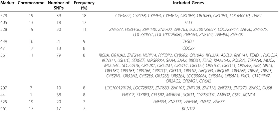
In addition to the results in Table 2, Table 3 reports information on the 10 most frequently significant mar-kers, as adjusted by the FDR control. Compared with Table 2, we find that the frequency (17 out of 199) of significant markers appearing in the 199 replicates is higher for the marker derived from the geneFLT1. The FDR control method increases the chance of detecting FLT1 but also increases type I errors for other false-positive markers. Six markers (405, 529, 528, 207, 439, and 361) overlap in both tables. There are four disagree-ments in each table, indicating the differences caused by different multiple testing adjustments.
Conclusions
The primary goal in handling rare variants in association studies is to transition the data from rare to common variants. We used the first phenotype replication to identify interactions among SNPs on the same chromo-some, using tree-based methods. Markers were then naturally defined from the detected interactions. Com-pared with previous work, this novel approach produces meaningful markers that are informed directly by the data, instead of combining groups of SNPs without con-sidering interactions. The other 199 replications of phe-notypes were then used to evaluate the set of constructed markers. We report the 10 most frequently significant markers in the 199 replications. The signifi-cance threshold was adjusted by either Bonferroni cor-rection or FDR control.
In addition to considering the binary phenotype Affected used in our work, we can also consider the continuous phenotypes (Q1, Q2, or Q4) in the regres-sion tree framework. The constructed markers would
not necessarily be bilevel. Instead, the constructed markers could be multilevel, according to the classifi-cation of terminal nodes. We make use of the repli-cates to evaluate the performance of the proposed method. In real data analysis, the goal is to apply, not evaluate, the method. For a real data set, we can first construct the tree from the real data and then generate more data sets under the null hypothesis by randomly permuting the affection status. Then, we can assess the significance of the markers in the tree of the real data on the basis of the distribution from the permutation data sets. We have used this technique effectively before [14].
Acknowledgments
This work is supported in part by National Institutes of Health (NIH) grant R01 DA016750 from the National Institute on Drug Abuse and NIH grant T32 MH014235from the National Institute of Mental Health. The Genetic Analysis Workshop is supported by NIH grant R01 GM031575. We would also like to thank the editor and reviewers for their constructive comments.
This article has been published as part ofBMC ProceedingsVolume 5 Supplement 9, 2011: Genetic Analysis Workshop 17. The full contents of the supplement are available online at http://www.biomedcentral.com/1753-6561/5?issue=S9.
Authors’contributions
YJ and HZ designed the study and carried out the data analysis. YJ, JSB, and HZ drafted the manuscript. JSB, RC, YH, and EN participated in data analysis. All authors read and approved the final manuscript.
Competing interests
The authors declare that there are no competing interests.
Published: 29 November 2011
References
1. Ji W, Foo JN, O’Roak BJ, Zhao H, Larson MG, Simon DB, Newton-Cheh C, State MW, Levy D, Lifton RP: Rare independent mutations in renal salt handling genes contribute to blood pressure variation.Nat Genet2008, 40:592-599.
Table 3 Ten most frequently significant markers (FDR control)
Marker Chromosome Number of SNPs
Frequency (%)
Included Genes
529 19 39 18 CYP4F22,CYP4F8,CYP4F3,CYP4F12,OR10H3,OR10H5,OR10H1,LOC646610,TPM4
405 13 18 17 FLT1
528 19 30 11 ZNF627,HSZFP36,ZNF440,ZNF700,ZNF763,LOC100129837,LOC729747,ZNF20,ZNF625,
LOC730651,LOC100129686,ZNF563,ZNF564,ZNF490,ZNF791
439 16 21 9 TPSD1
OR52N1,OR52N2,OR52E6,OR52E8,OR52E4,LOC390084,OR56A4,OR56A1,FXC1,C11ORF47,
OR2AG2,OR2AG1,OR6A2
207 7 10 8 LOC100129126,LOC728927,ZNF680,ZNF107,ZNF138,ZNF138,ZNF273,ZNF273,ZNF92,GUSB
44 1 38 8 FNDC7,STXBP3,CELSR2,MYBPHL,SORT1,CYB561D1,AMPD2,CSF1,KCNC4
525 19 20 7 ZNF554,ZNF555,ZNF556,ZNF57,ZNF77
2. Manolio T, Collins F, Cox N, Goldstein D, Hindorff L, Hunter D, McCarthy M, Ramos E, Cardon L, Chakravarti A,et al:Finding the missing heritability of complex diseases.Nature2009,461:747-753.
3. Nejentsev S, Walker N, Riches D, Egholm M, Todd JA:Rare variants of IFIH1, a gene implicated in antiviral responses, protect against type 1 diabetes.Science2009,324:387-389.
4. Dering C, Pugh E, Ziegler A:Statistical analysis of rare sequence variants: an overview of collapsing methods.Genet Epidemiol2011,X(suppl X):X-X. 5. Li B, Leal S:Methods for detecting associations with rare variants for
common diseases: application to analysis of sequence data.Am J Hum Genet2008,83:311-321.
6. Madsen B, Browning S: A groupwise association test for rare mutations using a weighted sum statistic.PLoS Genet2009,5:e1000384.
7. Morris A, Zeggini E: An evaluation of statistical approaches to rare variant analysis in genetic association studies.Genet Epidemiol2010, 34:188-193.
8. Wigginton JE, Cutler DJ, Abecasis GR:A note on exact tests of Hardy-Weinberg equilibrium.Am J Hum Genet2005,76:887-893.
9. Purcell S, Neale B, Todd-Brown K, Thomas L, Ferreira MA, Bender D, Maller J, Sklar P, de Bakker PI, Daly MJ,et al:PLINK: a tool set for whole-genome association and population-based linkage analysis.Am J Hum Genet2007, 81:559-575.
10. Dasgupta A, Sun YV, Konig IR, Bailey-Wilson JE, Malley J:A brief review of regression-based and machine learning methods in genetic
epidemiology: the GAW17 experience.Genet Epidemiol2011,X(suppl X): X-X.
11. Zhang H, Singer B:Recursive partitioning in the health sciences.New York, Springer; 1999.
12. Benjamini Y, Hochberg Y:Controlling the false discovery rate: a practical and powerful approach to multiple testing.J R Stat Soc Ser B Methodol
1995,57:289-300.
13. Almasy LA, Dyer TD, Peralta JM, Kent JW Jr., Charlesworth JC, Curran JE, Blangero J:Genetic Analysis Workshop 17 mini-exome simulation.BMC Proc2011,5(suppl 9):S2.
14. Chen X, Liu C-T, Zhang M, Zhang H:A forest-based approach to identifying gene and gene-gene interactions.Proc Natl Acad Sci USA
2007,104:19,199-19,203.
doi:10.1186/1753-6561-5-S9-S102
Cite this article as:Jianget al.:Novel tree-based method to generate markers from rare variant data.BMC Proceedings20115(Suppl 9):S102.
Submit your next manuscript to BioMed Central and take full advantage of:
• Convenient online submission
• Thorough peer review
• No space constraints or color figure charges
• Immediate publication on acceptance
• Inclusion in PubMed, CAS, Scopus and Google Scholar
• Research which is freely available for redistribution