Automatic Waveform Selection method for Electrostatic Solitary Waves
H. Kojima1, Y. Omura1, H. Matsumoto1, K. Miyaguti1, and T. Mukai2
1 Radio Science Center for Space and Atmosphere, Kyoto University, Uji, Kyoto, Japan 2 Institute of Space and Astronautical Science, Sagamihara, Kanagawa, Japan
(Received January 31, 2000; Revised June 19, 2000; Accepted June 13, 2000)
The present paper introduces the Automatic Waveform Selection (AWS) method for identifying the Electrostatic Solitary Waves (ESW) observed by Plasma Wave Instrument (PWI) onboard the Geotail spacecraft. Since the proposed method is based on the bit-pattern comparison, it does not require a lot of computer resources and the process speed is much faster than other pattern matching method using the First Fourier Transformation or the Wavelet transformation. We define the ESW index using the proposed AWS method. The ESW index allows us to perform statistical analyses by calculating it from a huge amount of Geotail data sets. We describe the detailed procedure of this new method for identifying the ESW waveforms and evaluate its efficiency. Further, we show one example of the statistical analyses conducted by using the AWS method, and discuss the result consulting the plasma electron measurements.
1.
Introduction
The main objective of the Plasma Wave Instrument (PWI) onboard the Geotail spacecraft is to investigate plasma wave phenomena in the geomagnetic tail region and to study the microscopic processes such as wave-particle interactions (Matsumotoet al., 1994a). One of the important achieve-ments of the Geotail PWI is the discovery of Electrostatic Solitary Waves (ESW) in the Plasma Sheet Boundary Layer (PSBL) by using the Wave-Form Capture receiver (WFC), which was newly designed for collecting waveforms of elec-tric and magnetic components up to 4 kHz (Matsumotoet al., 1994b). The ESW were initially reported as the wave-forms of Broadband Electrostatic Noise (BEN) observed in the PSBL. Since many theoretical attempts based on the ob-servations in the frequency domain have not succeeded in understanding the generation mechanism of BEN, the dis-covery of the ESW provided a breakthrough in the study of BEN.
The rapid progress of studies on the ESW have been made under the collaboration of spacecraft observations and
com-puter simulations. Matsumoto et al. (1994b) and Omura
et al. (1994) performed computer simulations on electron two-stream instabilities and pointed out that the ESW in the PSBL region correspond to electron holes in the velocity phase space and that such electron holes were produced as a result of nonlinear evolution of electron two-stream instabil-ities. They showed that the produced electron holes are very stable in time, which are equivalent to the Bernstein-Greene-Kruskal (BGK) mode (Bernstein et al., 1957). However, since such a two-streaming electron distribution is not re-alistic in the PSBL region, Omuraet al.(1996) examined electron distribution dependence of nonlinear evolutions of
Copy right cThe Society of Geomagnetism and Earth, Planetary and Space Sciences (SGEPSS); The Seismological Society of Japan; The Volcanological Society of Japan; The Geodetic Society of Japan; The Japanese Society for Planetary Sciences.
the electron beam instabilities by performing many simula-tion runs and they concluded that the most plausible genera-tion mechanism of ESW observed in the PSBL region is the electron bump-on-tail instability.
Other spacecraft observations in various regions of the magnetosphere confirmed that solitary waves similar to ESW observed by the Geotail are common plasma phenomena in space plasmas. First observations of solitary waves (struc-tures) were reported by Temerinet al. (1982). They were observed in the middle altitude of 6400 km in the polar at-mosphere by the S3-3 satellite. Further, after the discovery of the ESW by the Geotail, a series of new solitary waves has been observed in the polar region, solar wind, and bow shock by the Fast, Polar, Wind, and Geotail spacecraft (Matsumoto et al., 1997; Baleet al., 1998; Ergunet al., 1998; Franzet al., 1998; Mangeneyet al., 1999).
In order to confirm the generation mechanism proposed by computer simulations, we need to compare the observation results of ESW with the ESW properties predicted by com-puter simulations. However, the discussions only for a few selected events are not enough. In order to understand prop-erties of ESW, it is necessary to perform statistical analyses using observed waveform data. The statistical analyses on the ESW require to collect ESW waveforms among a huge amount of data sets as much as possible. Such a process is very tough when we pick up ESW waveforms one by one only with our own eyes. Therefore, we need to develop a method for selecting ESW waveforms automatically among a huge amount of observation data using numerical calculations.
The goal of the present paper is to develop the Automatic Waveform Selection (AWS) method for ESW observed by the Geotail spacecraft. The developed method should satisfy the following conditions:
1) The computer resources (CPU and memory) should be minimized so that a huge amount of data sets can be
496 H. KOJIMAet al.: AUTOMATIC SELECTION METHOD FOR ESW
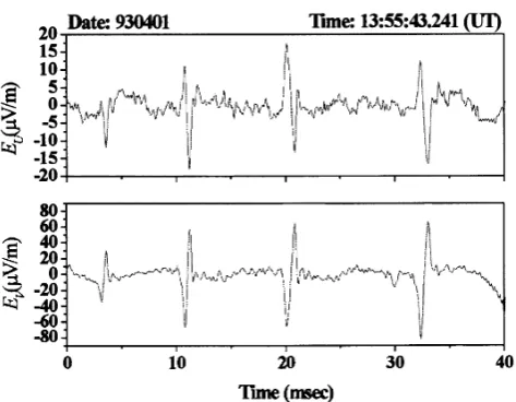
Fig. 1. An example of the Electrostatic Solitary Waves (ESW) observed in the Plasma Sheet Boundary Layer (PSBL). Upper and lower panels display the ESW observed by two sets of orthogonal electricfield dipole antennas with the length of 100 m tip-to-tip.
processed efficiently on a computational platform.
2) The selection should be correct as much as possible.
3) The method should yield information on amplitudes and pulse widths of the ESW as well as types of their wave-forms.
The AWS method which we describe in the present paper is very simple, but its efficiency is very high because it utilizes a bit-pattern comparison method instead of Fourier transfor-mation or Wavelet transfortransfor-mation, which are frequently used for pattern recognitions. Note that the detailed results of sta-tistical analyses on ESW using this method is described in Kojimaet al.(1999b).
Since the method which is described in the present paper is very general, it can be applied to other data sets which are observed by spacecraft, such as automatic selection of particular velocity distribution functions for ions/electrons.
2.
Electrostatic Solitary Waves
Figure 1 shows an example for the representative wave-forms of ESW observed at (GSM X, GSMY, GSM Z) = (−118, 4.3, 0.7RE) on April 1st, 1993. Two components of
waveforms shown in Fig. 1 are detected by two sets of orthog-onal electricfield dipole antennas with the length of 100 m tip-to-tip. Their characteristic pulse widths and inter-pulse widths are a few milliseconds and a few tens of millisec-onds, respectively. Matsumotoet al.(1994b) and Kojimaet al.(1997a) showed that these solitary waves correspond to isolated electrostatic potentials traveling along the ambient magneticfield.
Computer simulations using the full particle simulation code succeeded in reproducing waveforms of ESW (Matsumoto et al., 1994b; Omuraet al., 1994; Omura et al., 1996). They showed that ESW correspond to electron holes in the phase space and that they can be generated as the result of the nonlinear evolution of the electron bump-on-tail instability. Based on the computer simulation results,
the generation of ESW and their expected characteristics are summarized as follows:
1) The nonlinear evolution of Langmuir waves excited by electron bump-on-tail instability results in the forma-tion of isolated positively charged potential structures, which are equivalent to the BGK solution corresponding to electron holes in the velocity phase space.
2) Before reaching the final stage of the nonlinear evo-lution, the two-dimensional potential structure can be seen in the simulation space. However, the diffusion process due to electron cyclotron motion forces their two-dimensional structure to be reduced to the one-dimensional structure uniform in the direction perpen-dicular to the ambient magneticfield.
3) The generated isolated potentials travel along the am-bient magneticfield in the same direction of the elec-tron beam with almost the same velocity of the elecelec-tron beam.
In order to confirm the above results of computer simu-lations, we need to perform quantitative statistical analyses by collecting waveform data as many as possible. Since picking up ESW among huge amounts of Geotail waveform data needs tremendous efforts and time, we apply the pat-tern recognition method to select ESW waveforms from the Geotail data automatically.
There exist many kinds of useful methods based on the numerical calculations such as Fourier transformation or Wavelet transformation for identifying a specific pattern au-tomatically among data sets. However, since the total amount of data sets of Geotail waveform observations for the time period more than 7 years after the launch is very huge, we need to make use of the method, which does not require a lot of computer resources such as CPU power and size of mem-ories. Thus, we adopted a bit-pattern comparison method, which we introduce in the following section.
3.
Basic Concept
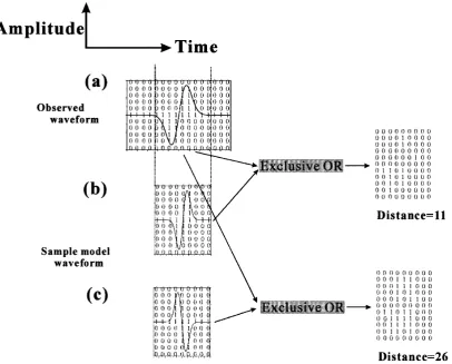
The automatic selection method for picking up ESW wave-forms, which we introduce in this section, is based on the bit-pattern comparison method. Figure 2 schematically il-lustrates this bit-pattern comparison method in the case of applying it for ESW.
Since the information of the phase of ESW waveforms is important in order to identify their traveling direction relative to the direction of the ambient magnetic field (details on identifying ESW traveling direction should be referred to Kojimaet al.(1999a)), we prepare two kinds of waveforms with opposite phase polarities as the sample ESW waveforms (see Figs. 2(b) and (c)). By comparing these two sample waveforms with observed Geotail waveform data (a) as the bit-pattern, we can identify the sample waveforms in the observed data by the following procedures.
Fig. 2. Basic concept of the bit-pattern comparison method. The bit-pattern comparison is conducted by calculating the Exclusive OR between the observed waveforms and the sample waveforms, which are prepared in advance.
2) Making a bit-pattern consisting of‘0’and‘1’for ob-served ESW waveforms.
3) Calculating Exclusive OR between the above two bit-patterns.
4) Calculating the number of‘1’in the result of the above Exclusive OR calculation (We address this number
“Distance”).
“Distance” represents how much the sample waveform resembles the observed waveform. When the sample wave-form completely corresponds to the observed one, the Dis-tance should be equal to zero. Thus, we can recognize the existence of ESW from small value of the Distance.
The above is the basic concept of the bit-pattern compar-ison method. In this method, since we do not make use of any complex calculation such as the Fourier transformation or Wavelet transformation, it does not require a lot of com-puter resources. Further, since the combination number on the result of Exclusive OR calculation between two patterns sampled withM bits in their amplitudes is very limited, we can prepare a table ofM×M matrices in advance and ob-tain the result of Exclusive OR only by accessing the table without any calculations in each step.
4.
ESW Index
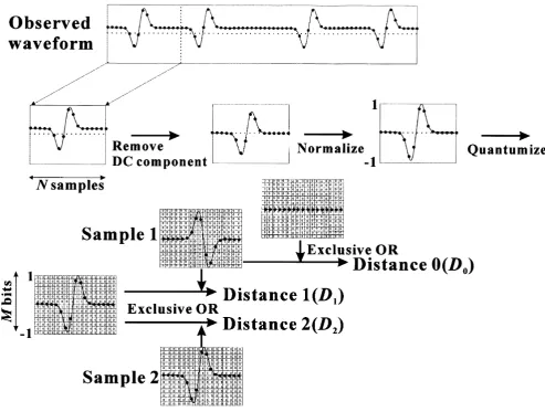
By using the above-mentioned method, we define the ESW index, which represents the existence of ESW type
wave-forms among the observed waveform data. The following procedure is conducted in generating the ESW index (see Fig. 3).
1) Cutting out the waveform data (x(i) : i = 1, . . . ,N) corresponding to N sample times from the observed waveform data.
2) Removing the DC (Direct Current) component by sub-tracting the average ofNsampled amplitudes as follow:
x(i)=x(i)− 1 N
N
j=1
x(j), i =1, . . . ,N. (1)
3) Searching for maximum absolute amplitude (Amax =
|x(i)|max). If the obtained maximum absolute
ampli-tude is less than the threshold level, which is specified in advance, we ignore the data set ofNpoints and skip the following procedure and examine the nextNdata.
4) Normalizing the data using Amax.
5) Quantumizing the amplitudes with M bits (in the pre-sent analysis, we quantumize the amplitudes in 64 bits (M =64)).
6) Performing the bit-pattern comparison and calculating the Distances (D1andD2) for two kinds of sample
498 H. KOJIMAet al.: AUTOMATIC SELECTION METHOD FOR ESW
Fig. 3. Schematic illustration on the procedure in obtaining the ESW index based on the bit-pattern comparison method.
7) Calculating the Distance (D0) between the Sample 1
and zero-level waveform (see Fig. 3).
8) UsingD0, we calculate the normalized Distances (D1
andD2) as follows:
D1,2= ⎧ ⎨ ⎩
1−D1,2
D0 ,
D1,2≤ D0
0 D1,2>D0.
(2)
9) FromD1 andD2, we obtain the ESW index as:
IESW=D1−D2. (3)
When we survey the time variation of the ESW index, we continue to perform the above procedure repeatedly for the observation data by shifting a sample waveform in time.
The ESW index means how much the observed waveforms resemble the prepared two sample waveforms with opposite phase polarities. The large positive or negative value of the ESW index means that the observed waveforms match the Sample 1 and Sample 2 waveforms, respectively.
In order to identify the ESW with different pulse widths, we need to compare observed waveforms with several sam-ple waveforms with different pulse widths. Therefore, we need to repeat the above procedure using different sample
waveforms in order to identify the ESW with different pulse widths. Since smaller number of sample waveforms to be compared is better in order to save the CPU time, in Section 6 we discuss the appropriate number of sample waveforms to be prepared in advance.
As we discuss in the later section, the information on the pulse width and peak amplitude of the ESW is very impor-tant. Since we search for the maximum amplitude in order to normalize observed waveform data (step 3 in the above pro-cedure), we can obtain the information on the positive and negative peak amplitudes of ESW and their time duration (τpp), simultaneously.
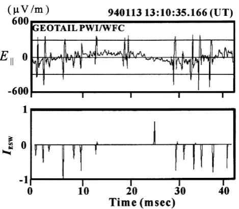
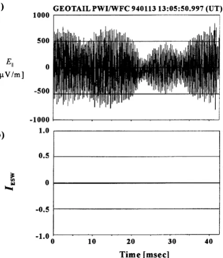
Figure 4 shows an example of identifying the ESW using the above AWS method. The upper panel shows the ob-served waveforms of electricfield component parallel to the ambient magneticfield (E). The data set shown in Fig. 4 is observed on January 13, 1994 at (GSM-X, GSM-Y,
GSM-Z) = (−95, 11,−4RE) and wefind that they contain many
ESW waveforms.
Fig. 4. Example of the time variation of the ESW index (lower) as well as corresponding waveforms (upper).
The ESW index misses identifying two ESW waveforms which appear at 13:10:35.184 (UT). This error is caused by the fact that the inter-pulse width between these two ESW is too short relative to their pulse widths. However, if we compare them with the sample waveform with a shorter pulse width, we can pick them up as the ESW waveforms.
5.
Definition of ESW Pulse Width
The sample waveform for ESW is generated under the approximation of Gaussian potential model (Krasovskyet al., 1997). The Gaussian potential structure and corresponding spatial waveform of electricfield are defined as
φ(z)=φoexp
−z2
λ2
, (4)
E(z)= −gradφ=2φo
λ2 zexp
−z2
λ2
. (5)
Thus, the sample model waveform of ESW in the time do-main is described as
E(t)=2φo λ
t τ exp
−t2
τ2
, (6)
whereτ = λ
V, andV is the velocity of ESW potentials. We
generate the sample model pattern of ESW from Eq. (6) (see Fig. 5).
The pulse width of ESW provides important information for evaluating potential scales and potential depths. The def-inition of the pulse width is ambiguous, but in our statistical analyses, we make use of the time interval (τpp) between two
peak amplitudes|Emax|of ESW waveforms for its defi
ni-tion because they are easy to be identified in the waveform data.|Emax|is obtained att = ±√τ
2 in the above Gaussian potential model (see Fig. 5). Thus, we define the pulse width (τESW) of ESW as three times of time interval of two peak
amplitudes as follow
τESW=3×2×√τ
2 =3×τpp. (7)
Fig. 5. The definition of the ESW pulse width (τESW). The ESW pulse
width is defined according to the Gaussian potential model (upper) as
τESW=3×τpp, whereτppis the time interval of two peak amplitudes
(lower).
Fig. 6. The dependence of the ESW index on various ratios between the pulse width of the ESW (s1msec) and the pulse width of sample ESW
waveform (s2msec).
6.
Response of the ESW Index to ESW with
Dif-ferent Pulse Widths
As we described in the Section 4, the ESW index is ob-tained by applying two sample waveforms with opposite phase polarities and same pulse width to a series of observed waveform data. However, since the ESW have various pulse widths, we need to prepare several kinds of sample ESW waveforms with different pulse widths. In order to prescribe the appropriate number of sample ESW waveforms, the re-sponse of the ESW index for ESW with various pulse widths should be investigated.
Figure 6 shows the dependence of the ESW index on var-ious ratios between the pulse width of the ESW (s1 msec)
and the pulse width of sample ESW waveform (s2 msec).
500 H. KOJIMAet al.: AUTOMATIC SELECTION METHOD FOR ESW
Fig. 7. The response of the ESW index to the Electrostatic Quasi-Monochromatic Waves (EQMW), which are the waveforms of the Nar-rowband Electrostatic Noise (NEN).
Wefind that the ESW index responds in the wide range of
s1/s2ratio. It is evident that the ESW index (IESW) reaches
the maximum value“1”ins1 = s2. As the ratio ofs1/s2
varies from the unity, the ESW index gradually decreases. From thisfigure, when the ESW index obtained from the sample waveform with one pulse width is beyond 0.3, we can identify the ESW with the pulse width ratio (s2/s1) from
0.5 to 1.82.
Based on the above result, the number of prescribed sam-ple ESW waveforms is decided. Since the ESW pulse width is typically equal to a few milliseconds to a few tens of mil-liseconds, we prepare 5 sets of sample waveforms with the pulse widths of 1.0, 2.0, 4.0, 8.0, and 16.0 msec. When we judge the existence of ESW by the ESW index beyond 0.3, we can identify the ESW with the pulse widths from 0.5 msec to 29.1 msec.
7.
Response of ESW to Other Waveforms
When we apply the AWS method to the Geotail data, we need to confirm the reliability of this method. The present section provides examples, which show that the ESW in-dex does not misread other waveforms as ESW waveforms. As we described in Section 3, the ESW index is defined for the waveforms of electricfield component (E) parallel to the ambient magnetic field. The typical plasma waves withEcomponent observed by Geotail in the geomagnetic tail region are the electrostatic waves which propagate along the ambient magneticfield. They are mainly classified into ESW, Electrostatic Quasi-Monochromatic Waves (EQMW) as waveforms of Narrowband Electrostatic Noise (NEN), and Modulated Electron Plasma Waves (MEPW) (Kojimaet al.,
Fig. 8. The response of the ESW index to the Modulated Electron Plasma Waves.
1997a; Kojimaet al., 1997b). Therefore, we need to confirm that the ESW index can distinguish ESW waveforms from these EQMW and MEPW waveforms.
Figures 7 and 8 show that the results in applying the AWS method to the waveforms of lobe EQMW and MEPW, respec-tively. The EQMW waveforms in the upper panel of Fig. 7 is observed in the tail lobe region on July 30, 1993 at (GSMX, GSMY, GSMZ) = (−112,−36, 19 RE). The continuous
sinusoidal waveforms are the typical waveforms (EQMW) of the NEN observed in the magnetosheath region (Kojima
et al., 1997a). Since in this case the oscillation period is about equal to one millisecond, we calculate the ESW index using the sample pattern with the pulse width of 1 msec. As shown in the lower panel, the response of the ESW index in this case is very low. Only small ESW index less than 0.25 can be seen. Since the threshold level for identifying ESW is IESW =0.3, the EQMW waveforms are not identified as
ESW waveforms.
The intense waves with amplitude modulations displayed in Fig. 8 is the MEPW observed in the lobe region close to the PSBL on January 13, 1993 at (GSM X, GSMY, GSM
Z) = (−95, 11, −4 RE). The frequency of the MEPW is
equal to the local electron plasma frequency. In this case, the frequency is about equal to 2 kHz and the oscillation period is 0.5 msec. Therefore, we apply the sample ESW waveform with the pulse width of 0.6 msec to these displayed waveforms. The response of the ESW index is shown in the lower panel. Wefind that the ESW index does not show any response to the MEPW waveforms.
demon-Fig. 9. Example of the statistical analyses on the ESW, which are conducted by using the AWS method. The positive and negative values in the horizontal axes represent the pulse widths (amplitudes in the lower panel) of the earthward and tailward traveling ESW, respectively. The present statistical analysis shows that both earthward and tailward traveling ESW can be observed in this event.
strate the high reliability of the ESW index defined in the present paper.
8.
Application of the ESW Index
The AWS method for ESW allows us to pick up ESW waveforms automatically among a plenty of waveform data without any complex procedures. In the present section, we apply this method to one event, which was observed on January 13, 1994 as one example in order to show the ability of this method (The detailed achievement on the ESW study based on the statistical analyses conducted by this method is discussed by Kojimaet al.(1999b)).
The Geotail was located in the distant tail region at (GSM
X, GSMY, GSM Z) = (−95, 11,−4 RE) on January 13,
1994. This event is introduced by Kojimaet al.(1999a) as an event that both earthward and tailward traveling ESW are observed in the relation to the slow mode shocks. Figure 9 is the histogram displaying the number of ESW identified by the present automatic selection method during one WFC sampling sequence starting from 13:10:35.086 (UT). The up-per and lower panels show the distributions of the identified ESW in their pulse widths and in their amplitudes, respec-tively. Further, positive and negative values in the pulse width and in the amplitudes represent those of the ESW traveling earthward and tailward directions, respectively.
As introduced by Kojimaet al. (1999a), this statistical analysis displays that both tailward and earthward travel-ing ESW are observed in this event. Further, while the pulse widths of earthward traveling ESW mainly fall into the range less than 3 msec, those of tailward traveling ESW are dis-tributed in the wider range less than 11 msec. This result is consistent with the observation model proposed by Kojima
Fig. 10. The electron reduced velocity distribution function observed by the plasma instrument (LEP) during the same period of Fig. 9 (upper panel). In the lower panel, the extracted electron beam components are shown. The existing two electron beam components correspond to the electrons trapped by the tailward and earthward traveling ESW potentials, respectively.
502 H. KOJIMAet al.: AUTOMATIC SELECTION METHOD FOR ESW
In this model, while the tailward traveling ESW is generated in the upstream region of the slow mode shock, which is lo-cated in the earthward side of the spacecraft, the earthward ones are emitted from the distant neutral point, which is as-sumed to exist aroundX = −100RE. Regarding this event,
although Kojimaet al.(1999a) introduced only representa-tive waveforms traveling in both directions, the present AWS method allows us to examine the statistical characteristics of this event as shown in Fig. 9.
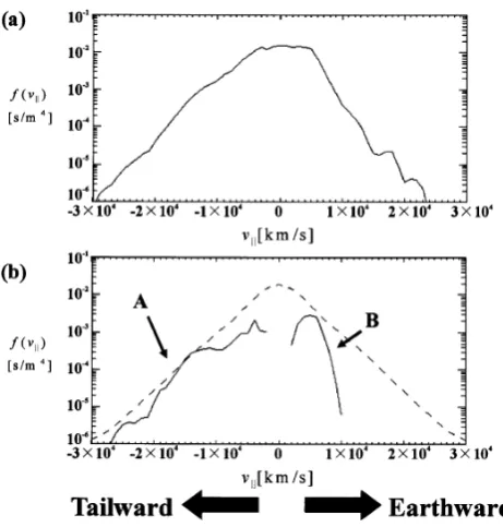
Figure 10 shows the reduced electron velocity distribution function (panel(a)) detected by Low Energy Particle exper-iment (LEP) in the same event (Mukaiet al., 1994). The tailward and earthward components correspond to the nega-tive and posinega-tive velocities, respecnega-tively. This reduced elec-tron distribution function possesses the evident high energy tail component in the tailward direction. Omuraet al.(1999) extracted“beam components”from this reduced electron ve-locity distribution as shown in Fig. 10(b). The main com-ponent of electron beams appears in the tailward direction and the slower beam component also exists in the earthward direction. These two electron beams seem to correspond to the tailward and earthward traveling ESW, respectively. Ac-cording to the ESW model as the electron hole in the phase space, which is proposed by Matsumotoet al.(1994b) and Omuraet al.(1994), the electrons trapped by ESW potentials produce high energy tail corresponding to their traveling di-rections in their velocity distribution functions. The results shown in Figs. 9 and 10 are very consistent with the ESW generation model.
9.
Summary
The present paper described the new method for selecting ESW waveforms automatically from a huge amount of the Geotail data sets. Since this method utilizes the bit-pattern comparison, the computer resources to be required are mini-mal, and its procedure is very simple. We can quickly extract the ESW waveforms from the data sets. Further, we can also obtain the information on their pulse widths and peak am-plitudes, simultaneously. This AWS method allows us to perform the statistical analyses on the ESW. As one ex-ample, the distribution of ESW pulse widths was presented, showing good agreement with the electron measurements. The quantitative analyses of the results using this method are presented by Kojimaet al.(1999b).
This method can be applicable to the data sets observed by other instruments as well as to other kinds of waveforms observed by the plasma wave receiver. The similar method was used in order to identify the shape of velocity distribution functions automatically in the Pioneer Venus mission (private communication with Crawford and Hammond). We can also apply this method to identify structures of the DC magnetic
fields or DC electric fields. We hope that the present new method of identifying the ESW waveforms is extended to other applications in this researchfield.
Acknowledgments. We would like to thank the ISAS/NASA Geotail mission project team for their support. We appreciate S. Kokubun and late T. Yamamoto providing MGF data to
iden-tify ESW propagation direction. We are grateful to G. K. Crawford and C. M. Hammond for introducing the bit-pattern comparison method, which was used in the Pioneer Venus mission. This re-search was supported by Grant-in-Aid for Scientific Research (A) 08404027.
References
Bale, S. D., P. J. Kellogg, D. E. Larson, R. P. Lin, K. Goetz, and R. P. Lepping, Bipolar electrostatic structures in the shock transition region: Evidence of electron phase space holes,Geophys. Res. Lett.,25, 2929–2932, 1998. Bernstein, I. B., J. M. Greene, and M. D. Kruskal, Exact nonlinear plasma
oscillations,Phys. Rev.,108, 546–550, 1957.
Ergun, R. E., C. W. Carlson, J. P. McFadden, F. S. Mozer, G. T. Delory, W. Peria, C. C. Chaston, M. Temerin, I. Roth, L. Muschietti, R. Elphic, R. Strangeway, R. Pfaff, C. A. Cattell, D. Klumpar, E. Shelley, W. Peterson, E. Moebius, and L. Kistler, FAST satellite observations of large-amplitude solitary structures,Geophys. Res. Lett.,25, 2041–2044, 1998. Franz, J. R., P. M. Kintner, J. S. Pickett, POLAR observations of coherent
electricfield structures,Geophys. Res. Lett.,25, 1277–1280, 1998. Kojima, H., H. Matsumoto, S. Chikuba, S. Horiyama, M. Ashour-Abdalla,
and R. R. Anderson, GEOTAIL Waveform Observations of Broadband/ Narrowband Electrostatic Noise in the Distant Tail,J. Geophys. Res.,102, 14439–14455, 1997a.
Kojima, H., H. Furuya, H. Usui, and H. sMatsumoto, Modulated electron plasma waves observed in the tail lobe: GEOTAIL waveform observa-tions,Geophys. Res. Lett.,24, 3049–3052, 1997b.
Kojima, H., K. Ohtsuka, H. Matsumoto, Y. Omura, R. R. Anderson, Y. Saito, T. Mukai, S. Kokubun, and T. Yamamoto, Plasma waves in slow-mode shocks observed by Geotail spacecraft, Adv. Space Res., 24, 51–54, 1999a.
Kojima, H., Y. Omura, H. Matsumoto, K. Miyaguti, and T. Mukai, Char-acteristics of electrostatic solitary waves observed in the plasma sheet boundary: Statistical analyses,Nonlinear Processes in Geophysics,6, 179, 186, 1999b.
Krasovsky, V. L., H. Matsumoto, and Y. Omura, Bernstein-Greene-Kruskal analysis of electrostatic solitary waves observed by Geotail spacecraft,J. Geophys. Res.,102, 22131–22139, 1997.
Mangeney, A., C. Salem, C. Lacombe, J.-L. Bougeret, C. Perche, R. Manning, P. J. Kellog, K. Geotz, S. J. Monson, and J.-M. Bosquend, WIND observations of coherent electrostatic waves in the solar wind, Annales Geophysicae,17, 307–320, 1999.
Matsumoto, H., I. Nagano, R. R. Anderson, H. Kojima, K. Hashimoto, M. Tsutsui, T. Okada, I. Kimura, Y. Omura, and M. Okada, Plasma wave observations with Geotail spacecraft,J. Geomag. Geoelectr.,46, 59–95, 1994a.
Matsumoto, H., H. Kojima, T. Miyatake, Y. Omura, M. Okada, I. Nagano, and M. Tsutsui, Electrostatic Solitary Waves (ESW) in the Magnetotail: BEN Wave forms observed by GEOTAIL,Geophys. Res. Lett.,21, 2915–
2918, 1994b.
Matsumoto, H., H. Kojima, Y. Kasaba, T. Miyake, R. R. Anderson, and T. Mukai, Plasma waves in the upstream and bow shock regions observed by Geotail,Adv. Space Res.,20, 683–693, 1997.
Mukai, T., S. Machida, Y. Saito, M. Hirahara, T. Terasawa, N. Kaya, T. Obara, M. Ejiri, and A. Nishida, The low energy particle (LEP) exper-iment onboard the Geotail satellite,J. Geomag. Geoelectr.,46, 669–692, 1994.
Omura, Y., H. Kojima, and H. Matsumoto, Computer simulation of Elec-trostatic Solitary Waves: A nonlinear model of broadband elecElec-trostatic noise,Geophys. Res. Lett.,21, 2923–2926, 1994.
Omura, Y., H. Matsumoto, T. Miyake, and H. Kojima, Electron beam in-stabilities as generation mechanism of electrostatic solitary waves in the magnetotail,J. Geophys. Res.,101, 2685–2697, 1996.
Omura, Y., H. Kojima, N. Miki, T. Mukai, H. Matsumoto, and R. Anderson, Electrostatic solitary waves carried by diffused electron beams observed by the GEOTAIL spacecraft,J. Geophys. Res.,104, 14627–14637, 1999. Temerin, M., K. Cerny, W. Lotko, and F. S. Mozer, Observations of double layers and solitary waves in the auroral plasma,Phys. Rev. Lett., 48, 1175–1179, 1982.