Exploration of Spatial and Temporal Changes in Trophic Status of Lakes in the Northern Temporal Forest Biome Using Remote Sensing

(1)

Electronic Thesis and Dissertation Repository

4-27-2015 12:00 AM

Exploration of Spatial and Temporal Changes in Trophic Status of

Lakes in the Northern Temporal Forest Biome Using Remote

Sensing

Aleksey Paltsev

The University of Western Ontario Supervisor

Dr. Irena I. Creed

The University of Western Ontario Graduate Program in Biology

A thesis submitted in partial fulfillment of the requirements for the degree in Master of Science © Aleksey Paltsev 2015

Follow this and additional works at: https://ir.lib.uwo.ca/etd

Part of the Biodiversity Commons, Biogeochemistry Commons, Environmental Monitoring Commons,

Forest Biology Commons, Fresh Water Studies Commons, Hydrology Commons, Other Earth Sciences Commons, Other Oceanography and Atmospheric Sciences and Meteorology Commons, Terrestrial and Aquatic Ecology Commons, and the Water Resource Management Commons

Recommended Citation Recommended Citation

Paltsev, Aleksey, "Exploration of Spatial and Temporal Changes in Trophic Status of Lakes in the Northern Temporal Forest Biome Using Remote Sensing" (2015). Electronic Thesis and Dissertation Repository. 2825.

https://ir.lib.uwo.ca/etd/2825

This Dissertation/Thesis is brought to you for free and open access by Scholarship@Western. It has been accepted for inclusion in Electronic Thesis and Dissertation Repository by an authorized administrator of

(2)

EXPLORATION OF SPATIAL AND TEMPORAL CHANGES IN TROPHIC STATUS OF LAKES IN THE

NORTHERN TEMPORAL FOREST BIOME USING REMOTE SENSING (Thesis format: Monograph)

by

Aleksey I. Paltsev

Graduate Program in Biology

A thesis submitted in partial fulfillment of the requirements for the degree of

Master of Science

The School of Graduate and Postdoctoral Studies The University of Western Ontario

London, Ontario, Canada

(3)

ii

Abstract

There is a critical need for detailed surveys of lakes covering large spatial

(>100 km2) and temporal scales (decades) to determine if there is an increase in the magnitude and frequency of phytoplankton blooms. Remote sensing was used to: (1)

develop a regression model that relates chlorophyll a (chl-a) as a proxy of lake

phytoplankton biomass to Landsat TM and ETM+ optical reflectance (r2=0.85,

p<0.001); and (2) apply this regression model to estimate chl-a in lakes within the

Temperate Forest Biome in Ontario over a 28-year period. A two-way Analysis of

Variance of remotely sensed chl-a of lakes revealed a spatial pattern of relatively low

chl-a in headwater lakes to higher chl-a in lower reaches of watersheds, and a

temporal pattern within a trend. These findings suggest that the recent increase in

community-driven reports of phytoplankton blooms is not indicative of an actual

increase in phytoplankton blooms in these lakes.

Keywords: temperate forest, lakes, trophic status, phytoplankton blooms,

(4)

iii

Co-Authorship Statement

Mr. Aleksey Paltsev will be the first author on any manuscript(s) submitted

from the contents of this thesis as he conducted satellite imagery data processing,

statistical analysis, and contributed to the design of the research approach. Dr. Irena F.

Creed will be a co-author on any manuscript(s) submitted from the contents of this

thesis as she contributed to the definition of the research problem, synthesis of ideas

and interpretation of the research results.

Financial support of the research activities for this project was provided by

Natural Sciences and Engineering Research Council of Canada (NSERC) Discovery

(5)

iv

Acknowledgments

First of all, I would like to thank my supervisor, Dr. Irena Creed, for all of her

guidance and encouragement throughout the entire 2.5 year research project. Dr.

Creed is an amazing scientist whose dedication to my professional development has

been invaluable and greatly appreciated.

I thank my advisory committee members, Dr. Katrina Moser, Dr. Hugh Henry

and Dr. Brian Branfireun, for allowing me the opportunity to accomplish this goal. Each member of my advisory committee contributed bright ideas that were

instrumental in making my thesis a success.

I thank Mr. David Aldred for his tremendous help in guiding me through

remote sensing techniques and developing automated scripts for satellite image

processing. I also thank Ms. Xue (Sherry) Qin for her incredible willingness to help as

well as for her support with satellite image processing and Ms. Jacqueline Serran for

her help with formatting text and numerous graphs in this thesis.

I would like to extend a special thanks to Dr. Eric Enanga who made my first

field trip in Canada unforgettable and from whom I learnt a lot on soil sampling. I

would also like to thank Dr. R. Sorichetti and Dr. G. Sass who became good friends of

(6)

v

List of Tables

Table 1.1: Overview of Landsat satellite sensors for phytoplankton monitoring (past

and currently operational) modified from Chander et al. (2009). RBV: Return Beam

Vidicon; MSS: Multispectral Scanner System; TM: Thematic Mapper; ETM+:

Enhanced Thematic Mapper; OLI: Operational Land Imager; pan: panchromatic; IR:

infrared; NIR: near infrared; SWIR: shortwave infrared; TIR: thermal infrared. ...7

Table 1.2: Overview of remote sensing studies using Landsat imagery for the

estimation of different parameters in inland waters only. B: Landsat band number;

LR: simple linear regression; MLR: multiple linear regression; Chl-a: chlorophyll-a;

SD: Secchi disk depth; TURB: turbidity; TSS: total suspended sediment; TSM:

total suspended matter; DOM: dissolved organic matter...9

Table 3.1: Correspondence between Landsat image capture dates and ground

measurement dates. ...21

Table 4.1: Descriptive statistics of in situ lake physical, chemical and biological data.

...30

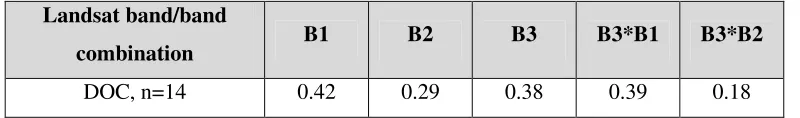
Table 4.2: Pearson correlation coefficients between in situ DOC and various Landsat

(9)

viii

List of Figures

Figure 1.1: Evidence for the increased number of phytoplankton blooms in southern

Ontario (modified from Winter et al., 2011). ...2

Figure 2.1: Location of the study region in the Temperate Forest Biome of Ontario

and the location of sampled lakes. ...16

Figure 3.1: Flowchart of Landsat TM and ETM+ image processing steps, lake

identification and reflectance calculation. ...22

Figure 4.1: Pearson correlation coefficients (r) between CHLaobs (ln [µg

CHLaobs/L]) and various Landsat bands, band combinations and band ratios...31

Figure 4.2: Relationship of time window between in situ and satellite observations

and r2, and number of lakes...33

Figure 4.3: Scatter-plot of B3 reflectance regressed against CHLaobs (ln [µg

CHLaobs/L])...35

Figure 4.4: Comparison of CHLaobs (ln [µg CHLaobs/L]) and CHLamod (ln [µg

CHLamod/L])...36

Figure 4.5: Map of average CHLamod (µg/L) for 21,384 lakes in a 28-year record....38

Figure 4.6: Time series of median CHLamod (ln [µg CHLamod/L]) for 6,384 lakes in a

28-year record (1984-2011) with an additional axis for CHLamod (µg/L)...39

Figure 4.7: Comparison in distribution of trophic status of lakes (%) for two ten-year

periods (1985-1994 and 1995-2004)...41

Figure 4.8: Sources of natural variation of CHLamod (ln [µg CHLamod/L]). ...42

Figure 4.9: Number of years needed to establish the stability of variance in CHLamod

(ln [µg CHLamod/L])...43

Figure 4.10: Number of lakes needed to establish the stability of variance in CHLamod

(10)

ix

List of Abbreviations

chl-a: Chlorophyll a

CHLaobs: Observed (sampled in the field) chlorophyll-a

CHLamod: Modelled chlorophyll-a

DOC: Dissolved organic carbon

TM: Landsat Thematic Mapper sensor

ETM+: Landsat Enhanced Thematic Mapper sensor

OLI: Operational Land Imager sensor

B1: Band 1 (Landsat blue band)

B2: Band 2 (Landsat green band)

B3: Band 3 (Landsat red band)

B4: Band 4 (Landsat near infrared band)

ANOVA: Analysis of variance

RMSE: Root mean square error

DOS - Dark Object Subtraction method

(11)

Chapter 1 1 Introduction

1.1 Problem Statement

Lakes in the temperate forests of eastern North America appear to be

experiencing an increase in the frequency and duration of phytoplankton blooms.

These blooms are often comprised of phytoplankton species that have the capacity to

produce toxic secondary metabolites such as neurotoxins, hepatoxins and

gastro-toxins that can cause serious health problems for animals and humans (Havens, 2008).

This has been the focus of numerous recent public and government reports (Winter et

al., 2011), resulting in heightened public concern and public reporting of

phytoplankton blooms in Ontario (Figure 1.1).

Phytoplankton blooms have usually been associated with the process of

eutrophication where excess macronutrients such as phosphorus (P) and nitrogen (N)

enter water bodies (Paerl and Huisman, 2009). The leading cause of this excessive

nutrient concentration is mainly ascribed to anthropogenic influences through either

direct discharge of waste products and chemical fertilizers into surface waters (Glibert

et al., 2005) or widespread land use and land cover change (e.g. deforestation, prairie plowing, wetland drainage, etc.) (Foley et al., 2005). However, these explanations

provide little or no insight into phytoplankton bloom occurrence in nutrient poor

oligotrophic lakes located on relatively pristine landscapes a considerable distance

from urban zones and agricultural lands.

Canada’s Great Lakes-St. Lawrence forest region contains 18% of the world’s

freshwater resources. With relatively little anthropogenic influence in the northern

parts of this region, it is likely that other factors are contributing towards a rise in

phytoplankton biomass. For example, climate warming and associated hydrological

and biogeochemical changes may be contributing to increased phytoplankton biomass

in oligotrophic lakes (O’Neil et al.,2012). More intense precipitation events promote

washing of nutrients out from uplands to wetlands and lakes, increasing their nutrient

enrichment. On the other hand, the prolonged periods of droughts lead to the effect

when nutrients are captured within lakes, raising a possibility of blooms (Paul, 2008;

(12)

Figure 1.1: Evidence for the increased number of phytoplankton blooms in southern

(13)

may indicate perceived rather than real concerns. An increased number of reports

does not necessarily indicate an actual increase in phytoplankton blooms. Public

perception may be heightened by a greater number of news stories illustrated with photographs of dead fish and livestock. Therefore, there is a critical need for a detailed historical survey of lake phytoplankton biomass covering large regional

scales over extended periods (decades) that can help determine whether global factors

such as climate change do play an important role and whether public perceptions are

accurate.

Until recently it was unfeasible to conduct this kind of research because it

required both comprehensive historical records and laborious sampling campaigns in

frequently difficult-to-access locations. The era of remotely sensed imagery, however,

allows for characterization of lake phytoplankton over large spatial extents over the

past several decades.

1.2 Theoretical framework for optical remote sensing of

phytoplankton

Satellite remote sensing has proven to be an effective tool for ecological

research in inland water bodies, helping to understand past and current complex

ecological and biogeochemical processes occurring in them. In lake science, the

application of remote sensing is based on the inherent properties of water, its

dissolved components, and phytoplankton pigments to absorb or reflect solar radiation

at specific wavelengths within the electromagnetic spectrum (Richardson, 1996).

The ability of a surface to reflect radiation is measured by reflectance; i.e., the

ratio of the total amount of reflected radiation (light) to the total amount of radiation

(light) incident on the surface. Every dissolved component or pigment in water has its

own reflectance properties, making it possible to “trace” their presence and

concentration in the water column. Phytoplankton detection is possible through the

optical properties of one of the principal pigments of all phytoplankton, chlorophyll a

(chl-a). Some phytoplankton groups have specific pigments, such as phycocyanin in

cyanobacteria with an electromagnetic absorption peak at about 620 nm, meaning that

these groups can be distinguished from other phytoplankton by their reflectance

(14)

phytoplankton bloom development and toxin production (Downing et al., 2001),

remote sensing promises to be a useful technique for studying these blooms via

detection of phycocyanin concentration in water. However, this technique is

hampered by the inability of most satellite sensors to resolve the narrow bandwidths

of these specialized absorption peaks and is still under investigation (Vincent et al.,

2004).

Among several currently existing remote sensing systems, one of the most popular and widely availablesystems is the Landsat satellite series. It offers the longest continuous record of satellite-based observations of the Earth’s surface starting with the launch of the first satellite in the series (Multispectral Scanner or MSS) in the early 1970s (Fraser 1998). Landsat Thematic Mapper (TM) and Enhanced TM (ETM+) sensors were subsequently launched to provide finer spatial

resolution (30 m). Landsat TM and ETM+ images consist of seven spectral

bands (with one additional band for ETM+) (Table 1.1). Table 1.1 presents an overview of all past and currently operational Landsat satellite sensors.

Landsat TM and ETM+ have a long history of successful quantification of

phytoplankton chl-a (Carpenter and Carpenter, 1983; Lathrop et al., 1991; Gitelson,

1992; Fraser, 1998; Allee and Johnson, 1999; Svab et al., 2005; Cannizzaro and Carder, 2006; Karakaya et al., 2011; McCullough et al., 2012; Hicks et al., 2013;

Giardino et al., 2014). These studies relied mostly on: (1) the optical properties of

chl-a chchl-archl-acterized by low reflectchl-ance in the red wchl-avelengths chl-and high reflectchl-ance in the

near-infrared; and (2) simple linear or multiple linear regression models where

satellite measured reflectance was related statistically to near-simultaneous

ground-based measurements of chl-a.

The successful use of Landsat TM and ETM+ imagery depends on various

factors, including the methods used for: (1) ground-based data collection (e.g., depth

from which a sample was collected); (2) correction of raw Landsat images to remove

terrain and atmospheric effects; and (3) statistical analysis (e.g., the type of regression

analysis used) (Liu et al., 2003;Kallio, 2012). It has also been shown that estimates

produced by regression models can be highly dependant on chl-a concentration;

accuracy can significantly drop with decreasing chl-a concentration (El-Alem et al.,

(15)

from remotely sensed imagery (using Landsat in particular) revealed that the majority

of models were developed from a single lake (e.g., Ritchie et al., 1990;Mayo et al.,

1995; Budd and Warrington, 2004; Vincent et al., 2004; Tebbs et al., 2013; Rodríguez

et al., 2014), some from a few lakes (e.g., Dekker and Peters, 1993; Gitelson, 1993;

Baruah et al., 2001; Brezonik et al., 2005), and only a handful from a large number of

lakes (e.g., Chipman et al., 2004; Olmanson et al., 2013) (Table 1.2).Few studies

have attempted to estimate chl-a over a period of more than one year (e.g., Kloiber et

al., 2002; Sass et al., 2007; McCullough et al., 2012; Hicks et al., 2013) (Table 1.2).

The studies that aimed at the model developing from many lakes

transferedknowledge from a few representative lakes to many lakes in a region. They

used in situ measurements from a few representative lakes to calibrate relationships

between Landsat TM or ETM+ imagery and chl-a, then extended the scale of study

from one year to decades and/or from small to large regions. For example, Pulliainen

et al. (2001) predicted average chl-aconcentration for lakes in southern Finland using

regression models developed from ground-based chl-a measurements in just six lakes.

The authors found that average chl-a can be reliably estimated from satellite data

(AISA hyperspectral system) without having in situ measurements for every lake.

Sass et al. (2007) classified trophic status in 76 lakes in northern Alberta (Canada),

finding a relationship between Landsat TM Band 3 (red) reflectance and ground

observations from 18 lakes (r2 = 0.68, p < 0.0001). Further, they used the regression equation and the reflectance derived from archived TM data to build a time series of

chl-a concentration for 20 years, thereby confirming the possibility of using remote

sensing of the lakes with no in situ data for continuous temporal analysis. Allan et al.

(2011) characterized the spatial and temporal distribution of chl-a in numerous lakes spread over the large area of the Central Volcanic Plateau in New Zealand, finding a strong relationship between Landsat ETM+ Band 3 reflectance values and in situ data (r2 = 0.95, p < 0.001). The developed model was transferred to predict the

concentration of chl-a for two different seasons (spring and summer) of the same year.

The previously mentioned studies have one particular idea in common: their models

(16)

Table 1.1: Overview of Landsat satellite sensors for phytoplankton monitoring (past and currently operational) modified from Chander et al.

(2009). RBV: Return Beam Vidicon; MSS: Multispectral Scanner System; TM: Thematic Mapper; ETM+: Enhanced Thematic Mapper; OLI: Operational Land Imager; pan: panchromatic; IR: infrared; NIR: near infrared; SWIR: shortwave infrared; TIR: thermal infrared.

Resolution

Satellite Sensors Launch Date

Decommission

Date _{Spectral Bands (B) (nm)} _{Pixel Size (m)} Revisit _Period (days) Altitude (km) Landsat 1 MSS and RBV July 23,

1972 January 7, 1978

80 (RBV)

79 (MSS) 18 920

Landsat 2 MSS and RBV January 22, 1975 February 25, 1982 RBV

B1 (green): 480-570 B2 (red): 580-680 B3 (NIR): 700-830

MSS

B4 (green): 500-600 B5 (red): 600-700 B6 (NIR): 700-800

B7 (SWIR): 800-1,100 80 (RBV) 79 (MSS) 18 920 Landsat 3 MSS and RBV March 5,

1978 March 31, 1983

RBV

B1 (pan): 505-750

MSS

B4 (green): 500-600 B5 (red): 600-700 B6 (NIR): 700-800

B7 (SWIR): 800-1,100 B8 (TIR):

10,400-12,600 40 (RBV) 79 (MSS) 240 (MSS thermal) 18 920

Landsat 4 MSS and TM

July 16,

1982 June 30, 2001 16 705

Landsat 5 MSS and TM

March 1, 1984

Completely deactivated: June 5, 2013

MSS

B4 (green): 500-600 B5 (red): 600-700

TM

B1 (blue): 450-520 B2 (green): 520-600

B3 (red): 630-690

82 (MSS) 30 (TM)

(17)

1,100 1,750 B6 (thermal IR):

10,400-12,500 B7 (SWIR-2):

2,080-2,350

Landsat 6 ETM+ October 5, 1993

Did not achieve

orbit 16 705

Landsat 7 ETM+ April 15,

1999 Operational

B1 (blue): 450-520 B2 (green): 520-600

B3 (red): 630-690 B4 (NIR): 760-900 B5 (SWIR-1): 1,550-1,750

B6 (TIR): 10,400-12,500 B7 (SWIR-2): 2,080-2,350

B8 (pan): 500-900

30 120 (thermal)

15 (pan)

16 705

EO-1 OLI November

21, 2000 Operational

B1 (coastal aerosol): 433-453 B2 (blue): 450-515 B3 (green): 525-600

B4 (red): 630-680 B5 (NIR): 845-885 B6 (SWIR-1): 1,560-1,660 B7 (SWIR-2): 2,100-2,300

B8 (pan): 500-680 B9 (cirrus): 1,360-1,390 B10 (TIR-1): 10,600-11,200 B11 (TIR-2): 11,500-12,500

30 100 (TIR)

15 (pan)

(18)

Table 1.2: Overview of remote sensing studies using Landsat imagery for the estimation of different parameters in inland waters only. B: Landsat band number; LR: simple linear regression; MLR: multiple linear regression; Chl-a: chlorophyll-a; SD: Secchi disk depth; TURB: turbidity; TSS: total suspended sediment; TSM: total suspended matter; DOM: dissolved organic matter.

Public

ation Location Sensor

# of modeled lakes # of years (period) Lake parameter Statistical technique Bands/band combinations/ band ratios r2 (chl-a only) Reference

2013 USA, Minnesota

TM, ETM+ 10500 20 (1985– 2005)

SD MLR B1/B3 n/a Olmanson et

al.(2013) 2013 New Zealand,

theWaikato region

ETM+ 34 9 (2000–

2009)

TSS, SD LR B4, B3, B1/B3 n/a Hicks et al., 2013

2012 USA, Maine TM, ETM+ 1511 20 (1990– 2010)

SD LR

(forward stepwise regression)

B1/B3 n/a McCullough

et al.(2012)

2011 New Zealand, Central Volcanic

Plateau

ETM+ n/a 1 (2001) Chl-a LR B3, B1/B3 0.95 Allan et al.

(2011)

2008 Southern Finland

ETM+ n/a 1 (2002) SD, TURB, DOM

LR B1/B3 n/a Kallio et al.

(2008) 2007 Canada,

Alberta, Boreal Plain

TM, ETM+ 76 20 (1984-2003)

Chl-a, SD, TURB

LR B3 0.68 Sass et al.

(2007)

2004 USA, Wisconsin

TM, ETM+ 8645 3 (1999– 2001)

SD MLR B1/B3, B1 n/a Chipman et al. (2004) 2003 USA, lower

peninsula of Michigan

ETM+ 93 1 (2001) SD LR B1/B3 n/a Nelson et al.

(19)

2003 USA, Minnesota

TM 94 1 (2001) SD MLR B1/B3, B1 n/a Sawaya et

al.

(2003) 2002 USA,

Minnesota, Twin Cities Metropolitan

Area

TM, MSS 64–170 25 (1973– 1998)

SD step-wise regression,

MLR

B1/B3, B1 n/a Kloiber et al.

(2002)

2002 The Netherlands,

Southern Frisian Lakes

TM n/a n/a TSM Analytical (B2 + B3)/2 n/a Dekker et al.

(2002)

2001 Southern Finland

TM 85 1 (1997) Chl-a, SD, TURB LR B1/B2, B1–B4)/ (B3– B1– B4)/(B3– B4), (B1– B4)/(B3– B4)

n/a Härmä et al.

(2001)

1998 USA, Nebraska Sand Hills,

Nebraska

TM 21 1 (1994) TURB LR B3 n/a Fraser

(20)

1.3 Analytical framework for optical remote sensing of

phytoplankton

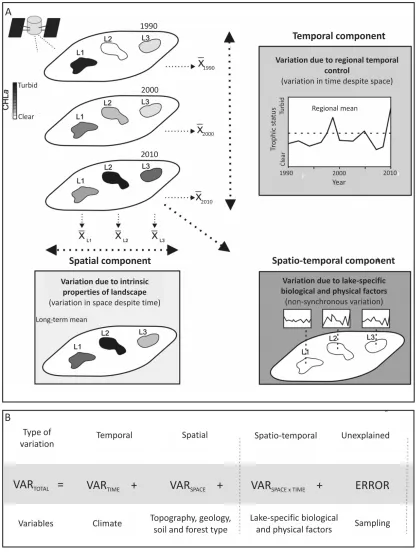
For this research the framework developed by Wiley et al. (1997) and later

applied by Sass et al. (2007) was adapted. Figure 1.2 shows schematic (A) and

statistical (B) models of three types of variation (space, time and space × time

interaction components) that contribute to overall variance in chl-a concentration.

Conceptually, the spatial component represents variation due to landscape attributes

of a study region including geology, topography, hydrology, forest and soil type (c.f.

Devito et al., 2005). Data on these attributes should be spatially extensive (Wiley et

al., 1997). For instance, they cannot represent concentration of chl-a for a single lake

but rather for many lakes in the region. The temporal component represents variation

due to differences between years including climatic oscillations and trends as well as

human development. Finally, the space × time interaction component represents

non-synchronous site (lake) specific variation in time. Processes leading to this type of

variation occur within lakes and can be biological (e.g., interactions between species

including competition and predation) or physical (e.g., morphometric properties of

lakes such as lake area, depth, size of littoral zone). The complexity of processes

involved in this type makes it difficult to define what exactly causes the variation.

Therefore, Sass et al. (2007) called it "variation due to unknown factors".

Statistically, all three components are integrated into the paradigm of standard

two-way analysis of variance (ANOVA). ANOVA has been widely used in ecological

research for evaluating spatial and temporal patterns with applications for

zooplankton (Lewis, 1978), fish and insect populations (Wiley et al., 1997), and chl-a

of eutrophic lakes (Sass et al., 2007). The spatial component represents averaged time

variation between sites, the temporal component represents averaged spatial variation

between years, while the space × time interaction component accounts for interaction

between time and space variations, namely variations that are site-specific (e.g. chl-a

that varies across the lakes of the same study region). Finally, the error term in the

ANOVA analysis may also be found in the space × time interaction component. This

error is associated with any measurement or remote sensing processing errors. It is

(21)

Figure 1.2: Schematic (A) and statistical (B) models of variation in the trophic status

(22)

time interaction component), but only if any replicates were collected during the

sampling period (Wiley et al., 1997).

1.4 Hypothesis and Objectives

The goal of the research is to characterize spatial and temporal variation in

lake chl-a as a proxy of phytoplankton biomass of lakes in the study region (the

northern edge of the Temperate Forest Biome) in Ontario.

The hypothesis is that concentration of chl-a in lakes in the Temperate Forest

Biome of Ontario is highly dependent on spatial and temporal differences in

topography and climatic patterns. The predictions are that: (1) the temporal

component of variation in chl-a is large, with an increase in chl-a over time related to

climate change; (2) the spatial component of variation in chl-a is similarly large, with

a systematic pattern of increase in chl-a from the upper to lower reaches of

watersheds; and (3) the space × time interaction component of variation is the

smallest.

To test this hypothesis, the following objectives were completed:

1. develop regression models that relate chl-a to optical reflectance;

2. apply these models to estimate chl-a concentration in lakes over several

decades;

3. decompose the total variation in chl-a into space, time, and space × time

interaction components to identify the main factors influencing chl-a

concentration.

The results of the study will help to identify which factors are associated with

reported phytoplankton blooms and allow researchers to target future monitoring

efforts on the potentially susceptible lakes in forested landscapes.

1.5 Thesis Organization

This thesis has been prepared in monograph format. The introduction (Chapter

1) provides an overview of the research problem and presents the theoretical and

analytical approaches to address the research problem. Chapter 2 outlines the study

region. The methods section (Chapters 3) describes methods used in the study.

(23)

influencing variation in chl-a. Chapter 6 summarises the major conclusions of the

work, discusses the anticipated significance of the study, and identifies future research

(24)

Chapter 2 2 Study Region

The study region is in the Great Lakes-St. Lawrence Forest region located at

the northern edge of the Temperate Forest Biome and confined by the administrative borders of the province of Ontario (Figure 2.1).

Climate is continental, with precipitation being influenced by lake effect from

the Great Lakes and local orographic effects in areas of high relief (Baldwin et al.,

2011). According to McKenney et al. (2011), mean annual precipitationin the study region for the period of 1981–2010 was 990 mm. Areas with maximum annual precipitation are located along topographic heights facing the Great Lakes, especially

in the Batchawana and Muskoka watersheds (1135 mm and 1150 mm respectively).

Average annual mean air temperature for 1981-2010 was +4.4 oC, varying between +7.0 oC in the south-east and 1.8 oC in the north (McKenney et al., 2011). The frost-free period greatly depends on the location; in more warm and humid south regions

this period normally extends from April to November while in the north it lasts from

May to September (Baldwin et al., 2011). Peaks in stream discharge occur during

snowmelt in March to April and again in September to November during autumn

storms (Mengistuet al., 2013).

Geology is the Precambrian rocks of the Canadian Shield. Bedrock geology is

primarily composed of silicate greenstone with small outcrops of more felsic igneous

rock (Ontario Geological Survey, 2003). In the south, these rocks are almost

completely covered with glaciofluvial outwash, whereas they come to the surface

throughout the Algoma Highlands and the north portion of the study region. The

outwash is 1-2 m in width and generally consists of two layers: sandy loam ablation

till and a compacted lower slit loam basal till (Ontario Geological Survey, 2003).

Topography varies from flats and depressions along the shores of lakes Superior and

Huron to hills and uplands (Algoma and Madawaska highlands, Batchawana

Mountains). Elevations range from 180 m to 650 m at the summit of Batchawana

Mountain with an average of 460 m (Baldwin et al., 2000). The most rugged

topography occurs in the Algoma Highlands where hills of mostly oblong forms with

(25)

Figure 2.1: Location of the study region in the Temperate Forest Biome of Ontario

(26)

Soils in the southern portion of the study region are thin and undifferentiated brunisols. Central and northern areas of the study region are represented by orthic ferro-humic podzols gradually thickening, differentiating, and increasing in organic content on topographic benches. Wetland areas are comprised of ferric humisols with highly humified organic deposits (Canada Soil Survey Committee, 1978).

The Great Lakes-St. Lawrence Forest region is the second largest forest region in Ontario and represents the transitional zone between deciduous and coniferous forests. Deciduous species are primarily comprised of sugar (Acer saccharum Marsh.) and red (Acer rubrum L.) maples, yellow birch (Betula alleghaniensis Britt.), and red

oak (Quercus rubra L.). Coniferous species are represented by white (Pinus strobes

L.) and red (Pinus resinosa Ait) pine, and easternwhite cedar (Thuja occidentalis L).

There is a long history of forest management activities that have resulted in a fairly

simple forest structure, with reduced species diversity and little variety in forest age

(Carleton, 2000). In addition, logging has also led to significant changes in nutrient composition of local soils (especially nitrogen [N] and dissolved organic carbon [DOC]) that could have had potential impact on the streams and lakes of the study

(27)

3 Methods

3.1 Ground-based data

Ground-based measurements were taken as a part of the field campaign

launched in 2008 and conducted by Sorichetti (2013b). The measurements of

chlorophylla andDOC were made in 31 oligotrophic lakes in the Algoma Highlands of Ontario from 2009 to 2011 (Figure 2.1).Lakes were selected on a basis of minimal

direct anthropogenic influence and public concern about the potential of

phytoplankton blooms in the lakes.The sampled lakes are relatively deep (ranging

between 0.8 m to 42.7 m; Sorichetti, 2013b), thermally stratified during the warm

summer months, and dimictic with major mixing events occurring during the spring

snowmelt and fall storms. Lakes were sampled at their centers throughout the ice-free

season (May – October). Surface water samples integrated to 1.0 m depth were

collected in 500 mL pre-rinsed polyethylene bottles near the centres of the lakes. The

samples were then put into in a cooler with ice until return to the field laboratory.

Each sample was filtered onto Whatman GF/F filters and analysed for chl-a

concentration according to EPA Method 445.0 (Arar and Collins, 1997). Chl-a was

extracted from filters using an acetone/ultra-pure water solvent (90:10 v/v) in 20 mL

scintillation vials and stored in the dark at -20 °C for 20 h. Samples were brought to

room temperature in the dark and measured using a Turner 10-AU field fluorometer

with a 680-nm emissions filter (Turner Designs, Sunnyvale, CA, U.S.A.).

Ground-based measurements of chl-a conducted by Sass et al. (2007) were

also used in this study. The measurements were taken in 22 eutrophic lakes in August

2001 in the Boreal Plain in northern Alberta. The lakes were relatively shallow with

an average depth of 1.3 m (Sass et al., 2008). Lakes were sampled at their centers in

mid-August coinciding with the summer peak in phytoplankton biomass. Grab

samples were taken from a depth of 0.20-0.40 m of the water column and transported

to a laboratory. Samples were filtered within 12 hours of collection, frozen, and later

analyzed for chl-a using a spectrophotometer at 750, 665 and 649 nm using EPA

(28)

(2007). Satellite reflectance values for the Alberta lakes were also provided by Sass et

al. (2007).

3.2 Satellite-based data

3.2.1 Rationale for choosing Landsat TM and ETM+ imagery

Archived Landsat TM and ETM+ satellite images were chosen as the source

of satellite-based data for this research for a number of reasons: (1) well-established

methods of image and associated metadata processing; (2) near-continuous coverage

of archived satellite imagery starting from 1982; (3) global coverage allowing for

analysis over large areas as well as in areas with limited or no physical access; and (4)

free distribution, an especially important consideration for historic surveys of large

areas with requirements of hundreds thousands of scenes.

3.2.2 Landsat data acquisition

Twelve Worldwide Reference System ground tracks (path and row

combinations 22/27, 21/28, 20/27, 20/28, 17/28, 17/29, 16/29, 18/28, 18/29, 21/27,

19/27, 19/28; UTM zones 16, 17 and 18) were identified for the study region. Landsat

TM (1984-2011) and ETM+ (1999-2003) scenes as well as associated metadata

corresponding to these tracks were retrieved from US Geological Survey archives for

the period of 1984-2011. ETM+ images for the period of 2003-2011 were not

acquired due to a system failure in the Landsat 7 sensor in 2003 that resulted in wide

strips of missing data within images. Only those images were selected that: (1)

contained less than 50% cloud or haze cover; and (2) were captured from late July to

early November. This period coincides with the peak phytoplankton biomass known

for the study region, extending into a prolonged autumn boundary. This boundary

may extend into ice cover periods, but it was set this way intentionally due to new

evidence that duration of phytoplankton blooms is increasing, covering a period up to

mid-November (Winter et al., 2011).

Although the 16-day revisit period of Landsat satellites offers the potential to

acquire two images for each ground track in most months, the presence of cloud cover

limited this number; in many months no usable images could be acquired. Particular

(29)

and ground observation within +/- 7 days was used to limit the search. Although this

window is the longest period in which reasonable results can be yielded (Kloiber et al,

2002; Nelson et al., 2003), it remained a challenge to find cloud-free Landsat images

falling within this window.

A total of 1,067 Landsat TM and 159 ETM+ images were retrieved. Five

images coinciding with the in situ measurements in 2009, 2010 and 2011 within +/- 6

days were acquired (Table 3.1). All images were corrected for terrain at delivery.

Landsat images were imported into ArcGIS 10.2 where they were cropped to remove

“dark” or zero value pixels on image margins. Only Bands 1-5 (out of 7) were

processed and used in this analysis.

3.2.3 At-satellite radiance calibration

Landsat images are stored in 8-bit Digital Numbers (DNs) for the purpose of

minimizing storage volume. This storage process involves scaling and offsetting the

physical at-satellite radiance values (the amount of energy sensed by the satellite

measured in W m-2 sr-1µm-1). The first step in image analysis is to convert DNs for each image Band 1-4 back to at-satellite radiance values (Lsat) using Equation 1:

[1]

where B and G are published post-launch image gain and bias provided in image

metadata (Chander et al., 2009). An automated script was developed for

implementation in ArcGIS 10.2 to execute at-satellite radiance calibration. Figure 3.1

shows a flowchart of Landsat processing.

3.2.4 Atmospheric correction

Estimating phytoplankton biomass or other water quality variables from

Landsat images depends on being able to relate Landsat pixel values to inherent

physical optical properties of the variables. Because these physical properties do not

vary in space or time, Landsat images acquired over a span of time and across

different ground tracks must be corrected to a common radiometric scale in order to

(30)

Table 3.1: Correspondence between Landsat image capture dates and ground

measurement dates.

Date of image

capture Sensor

Ground measurement date

May 22, 2009 TM May 17, 2009

June 12, 2009 TM June 13, 2009

June 23, 2009 TM June 24, 2009

June 17, 2010 TM June 16, 2010

August 16, 2010 TM August 16, 2010

(31)

Figure 3.1: Flowchart of Landsat TM and ETM+ image processing steps, lake

(32)

A major source of error is the modification of electromagnetic radiation

signals collected by satellites from scattering and absorption by gases and aerosols as

the signals travel through the atmosphere from the Earth’s surface. Atmospheric

interference can be particularly significant over water bodies, because interference

increases as reflected radiance from water decreases (Brezonik et al. 2005).

Atmospheric conditions vary in both space and time. The effects of atmospheric

conditions depend on the wavelength of energy reaching the given satellite sensor.

The main atmospheric effect is scattering which is additive to the remote sensed

signals, while the effect of absorption is multiplicative.

A number of methods have been developed to correct satellite images for

atmospheric effects (Chavez, 1996; Chen et al., 2005). Physical models are the most

complex and require detailed knowledge of atmospheric conditions such as Rayleigh

atmosphere, aerosols and ozone optical depth at the time of image acquisition. As

these parameters are rarely available – especially for historic and rural archived

imagery – physical models can typically only be used for field-calibrated studies

where in situ measurements can be made.

Relative methods use histogram matching and regression techniques to

normalize images to a single reference image by selecting pseudo-invariant ground

features (PIFs) that are assumed to have constant reflectance properties (Schott et al.,

1988; Furby et al., 2001). Relative methods are not applicable when generalization of

spectral features takes place across more than one Landsat frame as PIFs cannot be

identified across ground tracks (Mahiny et al., 2007).

Dark Object Subtraction methods (DOS) can be used across different scenes

and do not require in situ atmospheric measurements. These methods assume that

there are near-zero reflectance features ("dark features") within an image (e.g., clear

water bodies, dense forest, shadows) and that the signal recorded by the sensor is

solely a result of atmospheric scattering (path radiance) – this value is subtracted from

all pixels in an image (Shunlin et al, 2001). The Cosine of Sun Zenith Angle model

(COST) variation of DOS was adopted for this study (Chavez, 1996).

“Dark feature” DNs (DNmin) were identified by examining a histogram of DNs

in each image band. Only Bands 1-4 were processed and used in this analysis. The

(33)

Earth-Sun distance and solar zenith angle in addition to atmospheric effects by

converting physical at-satellite radiance values (Lsat) to unitless [0-1] surface

reflectance values (ρ) using Equation 2 (Chavez, 1996):

[2]

where:

a) d is the earth-sun distance in astronomical units (provided in lookup tables

according to image capture date);

b) Lp is dark object radiance ((Lp = DNmin – B / G) minus radiance contributed by

a percentage of surface reflectance (0.01 (1%) is an assumption of dark object

surface reflectance for Bands 1-3; 0.001 (0.1%) for Band 4; and 0 (0%) for

Band 5 (Lu et al., 2002; Mather and Tso, 2009; Clark et al., 2010));

c) Tv is atmospheric transmittance from target to sensor (assumed to be 1 by Lu et al., 2002);

d) Esun is an exoatmospheric solar constant (provided in lookup tables according

to satellite sensor);

e) ϴz is solar zenith angle in radians (published in image metadata); and

f) Tz is atmospheric transmittance in the illumination direction from sun to target

(given as ϴz for Bands 1-4).

An automated script was developed for implementation in ArcGIS 10.2 to

execute atmospheric correction for all images.

3.2.5 Lake identification

Pixels representing water bodies were identified according to an approach

suggested by Frazier et al. (2003). A threshold value between water and non-water

pixels for each image was identified by analysing histograms of raw Band 5

(shortwave infrared) DNs for each image (a band in which radiation is strongly

absorbed by water). This value was then used to reclassify the Band 5 images where

pixels were assigned as water below this threshold and values equal to and above the

(34)

Water pixels were then converted to polygons. Since the water pixels

accounted for not only lakes but also for other water features such as rivers and

streams, these polygons were manually removed, thereby leaving only lakes (the

“satellite lakes”) for further analysis.

Cloud/shadow masks were generated automatically from the raw Landsat DNs

by applying a stand-alone software package Fmask 3.2 (“Function of Mask”) that was

initially developed by Zhu and Woodcock (2012) as a Matlab code. Fmask uses the

physical properties of clouds (e.g., temperature, brightness) and the darkening effect

of cloud shadows in the near infrared band (Band 4) to separate cloud/shadow pixels

and clear sky pixels. Fmask can also be used to detect snow pixels – this function was

particularly important for analyzing images captured in late October – November.

Lake polygons intersecting any pixels classified as cloud, shadow or snow were

discarded.

3.2.6 Lake selection for regression modeling

Sass et al. (2007)cite the importance of lake selection criteria when dealing

with prediction of chl-a for small lakes because of potential errors appearing in pixels

near or along lake shorelines. The reflectance properties of shallow water and/or

abundant emergent or aquatic vegetation that appear at the edges of water features are

different than those of deeper water, producing pixels with mixed reflectances.

In order to avoid this problem, a minimum lake area of 4.5 ha (50 digital

pixels for images with 30 m resolution) was applied – lake polygons with a smaller

area were discarded. The remaining lake polygons were buffered inside to a distance

of 15 m (1/2 pixel distance), further reducing the potential effects of mixed pixels.

Mean reflectance values for each Landsat Band 1-4 were extracted within each

buffered lake polygon.

Twenty-six of 31 ground sampled lakes were matched with satellite lakes,

meaning that seven ground sampled lakes were either: (1) cloud covered at the time of

image capture; (2) smaller than 4.5 ha; or (3) image capture fell outside the +/-7 day

window of ground observation. Nine of the 26 ground sampled lakes had in situ chl-a

(35)

within a +/- 6 day time window of image capture.

3.2.7 Regression modeling

Ground-based measurements of chl-a were related to mean lake reflectance.

Pearson correlation was used to determine statistical relationships between natural log

transformed ground-based chl-a (hereafter referred to as CHLaobs) and reflectances

from Landsat bands (B), band combinations and band ratios. Band combinations and

band ratios were chosen on the basis of a review of studies (Dekker and Peters, 1993;

Chen et al., 1996; Vincent et al., 2004; Hellweger et al., 2004). Twenty-one different

bands, band combinations and band ratios were tested to determine the strongest

relationship of reflectance to chl-a by comparing with CHLaobs using the Pearson product-moment correlation coefficient (r). This correlation had already been

conducted on the CHLaobs from the Alberta lakes.

The Pearson correlation coefficient was also used to test potential relationships

between natural log transformed DOC sampled in the Ontario lakes and reflectance

values to determine whether DOC had any confounding effect on reflectance.

Sass et al. (2007) found that a maximum +/- 2 day time window between

ground measurement and image capture was optimal for their model. To determine

this window for the Ontario lakes, simple linear regressions between reflectance (in

the band, band combination or band ratio determined to have the strongest

relationship with CHLaobs) and CHLaobs for each time window interval step of one

day between +/ 1 to +/- 6 days. A maximum +/- 3 day time window left a total of 31

Ontario lake samples.

Ontario and Alberta ground sampled lakes were combined into a single dataset

for modeling. Cook's distance of CHLaobs was calculated in three iterations to identify and eliminate six outliers, leaving 47 samples for use in modeling. The resulting

dataset was randomly split into two datasets of 24 and 23 lakes covering

approximately the same ranges of chl-a and reflectance in the band, band combination

or band ratio determined to have the strongest relationship with CHLaobs. The first

(36)

A linear regression model was developed from the first dataset of 24 lakes

using CHLaobs as the dependent variable and the band, band combination or band ratio

determined to have the strongest relationship with CHLaobs as the independent

variable. The equation obtained from the regression model was applied to predict

chl-a (herechl-after referred to chl-as CHLchl-amod) for the lakes in the model validation dataset. A linear regression was conducted using CHLaobs from the validation dataset as the

dependent variable and CHLamod as the independent variableto determine the strength

of the model and to confirm that predicted values fit onto a 1:1 line with no intercept

with observed values. The model equation was then applied to all lakes in each

Landsat image and for the entire period of 1984-2011. These remaining images

included 793 cloud-free processed images from the end of July to mid-November with

the highest number of them captured in August and September (around 70%).

A total of 21,384 satellite lake observations were found to be located within

the study region over the 28-year period. These lakes were used for evaluating spatial

distribution of CHLamod within the study region as well as for analysing their trophic

status. However, many of these lakes lacked complete CHLamod data for some years

due to haze and clouds. In order to build temporal patterns where the development of

chl-a over a 28-year period could be identified, it was important to have a continuous

annual record of CHLamod for the same lakes. Therefore, lakes with missing data (i.e.

missing years) were excluded, leaving a final selection of 6,384lakes.

3.2.8 Decomposition of variance

Two-way analysis of variance (ANOVA) was used to evaluate spatial and

temporal patterns in CHLamod (Figure 1.2B). The variation in CHLamod was

decomposed into space, time and space × time interaction components, statistically

expressed as the sum of squares in space (SSspace), time (SStime), and space × time

(SSspace x timet). The ANOVA matrix consisted of 28 columns corresponding to the

number of years and 6,384 rows corresponded to the number of lake records. The

space factor accounted for evaluation of the difference between the 28-year average

CHLamod for a specific lake and the 28-year average of all lakes, whereas the time

factor accounted for the difference between the average CHLamod of all lakes for a

(37)

space and time factors (SStotal - SSspace - SStime).

ANOVAs were also conducted on subsets of the dataset to examine the

stability of variance in CHLamod with gradually increasing temporal and spatial extent

of sampling (i.e., the effect of number of years and number of lakes). Twenty subsets

were selected for testing both the number of years and the number of lakes. While

testing the effect of the number of years: (a) ANOVAs were performed for every year

from 1985 to 1997 and for every two years from 1998 to 2011; and (b) all 20 subsets

consisted of 6,384 lakes. While testing the effect of the number of lakes: (a) ANOVAs

were performed on subsets containing between 200 and 6384 lakes increasing in size

by increments of 200 between 200 and 2000 lakes and of 400 between 2001 and 6384

lakes; and (b) all 20 subsets consisted of 28 years. In the end, two final datasets were

created (number of years and number of lakes) with proportions of total variation in

CHLamod (in percentages).

The minimum number of years and lakes which was required to establish the

stability of variance in CHLamod was determined by identifying breakpoints for each

of three components (i.e., space, time and time x space interaction) with the use of

nonlinear piecewise regressions. Since the breakpoints for each component were

different, the one with maximum value (i.e., number of years or number of lakes) was

(38)

Chapter 4 4 Results

4.1 Chl-a concentration in ground-based samples

CHLaobs in 24 lakes selected for the regression model development ranged

from 0.50 to 78.79 µg/L with an average of 14.51 µg/L (Table 4.1). CHLaobs in the 23

lakes selected for the validation dataset ranged from 0.39 to 59.6 µg/L with an

average of 12.1 (µg/L). This indicates that both datasets represented the lakes of all

trophic states from oligotrophic to hypereutrophic (very nutrient rich; Carlson and

Simpson, 1996).

4.2 Regression model

Analysis of reflectance values showed that bands B2 (green) and B3 as well as

band combinations B3*B1 and B3*B2 were significantly correlated to CHLaobs in the

Ontario lakes with B3 showing the strongest correlation (r=0.91, p < 0.0001; Figure

4.1). Similar coefficients were found by Sass et al. (2007) for Alberta lakes (B3, PCC

= 0.82, p < 0.0001). Therefore, this band was chosen for the regression model

development. It was interesting to find that band ratio B3*B1 also had significant

correlation reaching a mark of 0.90 (p < 0.0001). There were no previous studies

found having any comparable results for this ratio for inland waters.

The possible contribution of DOC to the strength of the regression model was

considered. DOC absorbs moderately in the red wavelengths (B3) leading to potential

changes in the spectral reflectance properties (Gitelson et al., 1993, Svab et al., 2006).

However, there was no significant relationship found between this band and DOC (r=

0.38, p = 0.18, n = 14; Table 4.2).

A series of linear regression models were developed of CHLaobs from the

Ontario lakes and B3 by successively increasing the time window between the day of

image capture and sample day in one day increments from +/- 1 to +/- 6 days (Figure

4.2). As the time window increased, the strength of relationships decreased (r2

decreasing from 0.82 to 0.21 with increasing time windows). There was a significant

drop in the strength of relationships after +/-3 days (r2 decreasing from0.73 for

(39)

Table 4.1: Descriptive statistics of in situ lake physical, chemical and biological data.

n Mean Min Max Median

CHLaobs (µg/L)* 24 14.51 0.50 78.79 3.71

DOC (µg/L) 14 5148.68 2634.00 8477.90 4368.26

Validation CHLaobs

(µg/L) 23 12.1 0.39 59.60 5.59

(40)

(41)

bands and band ratios.

Landsat band/band

combination B1 B2 B3 B3*B1 B3*B2

(42)

Figure 4.2: Relationship of time window between in situ and satellite observations

(43)

strength of their models from one time step to another owing likely to a far larger

sample size (160 lakes in contrast to 35). Given the relative strength of the

relationship found using a time window of +/- 3 days, the decision was made to use

this time window to preserve a relatively large number of sample lakes (31).

Cook's distance identified six outliers in our dataset. Four of them came from

Ontario dataset from 2011, while two came from the Alberta dataset. The fact that all

the outliers from the Ontario dataset were from the same year suggests that this year

may have been exceptional in terms of climatic conditions.

A linear regression model performed using CHLaobs from the 24 lake model

development dataset explained 85% of variation in CHLamod (r2 = 0.85, p < 0.001, n =

24; Figure 4.3). 23 out of 24 lakes fell within the bounds of 95% prediction limits.

4.2.1 Results validation

The accuracy of model was assessed using the validation dataset of 23 lakes

(Table 4.1). The comparison revealed significant correlation between CHLaobs and

CHLamod with a root mean square error (RMSE) = 0.55 (r2 = 0.84 and p < 0.0001;

Figure 4.4). The slope of the regression was found to be only slightly greater than 1

(1.0079) and the intercept only slightly less than 0 (-0.0997). Therefore, it was

concluded that the predictive power of the model was good.

4.3 Spatial patterns in modelled chlorophyll a

Spatial patterns were assessed on the basis of a trophic status map of 21,384

lakes (Figure 4.5). The map was created by averaging the 28-year record of CHLamod

for each lake. This average concentration was used to classify the lakes into four main

trophic groups according to Carlson and Simpson (1996): oligotrophic, mesotrophic

(intermediate nutrient levels), eutrophic (nutrient rich) and hypereutrophic. The map

revealed two distinct patterns in average CHLamod.

First, lakes located in close proximity (within 100 km) to Lakes Superior and

Huron are mostly mesotrophic or eutrophic. Further, most of the highly productive

hypereutrophic lakes (CHLamod > 56 µg) of the study region are also found in close

proximity to the Great Lakes (especially to the northern shore of Lake Huron and Saul

(44)

Figure 4.3: Scatter-plot of B3 reflectance regressed against

(45)

Figure 4.4: Comparison of CHLaobs (ln [µg CHLaobs/L]) and

(46)

of the region. The distribution of mesotrophic and eutrophic lakes is apparently more

random.

Second, oligotrophic lakes are concentrated along the topographic divides

between watersheds. They form an almost continuous "oligotrophic belt" with the

only interruption in the south-eastern portion of the region.

4.4 Temporal patterns in modelled chlorophyll a

A 28-year time series of annual median CHLamod for 6,384lakes was created

for the analysis of temporal patterns (Figure 4.6).

The time series revealed a cyclic structured pattern in the median CHLamod

with a different range and intensity of fluctuation over the 28-year period. The range

of fluctuation seems to be higher between 1989 and 1999. The time series also

revealed three peaks in the median CHLamod in 1991, 2000 and 2010 with

approximately the same CHLamod (7.5 µg/L).

4.5 Alterations in the trophic status of lakes

The bar chart of comparison in the proportions of lakes trophic status for two

periods showed an increasing trend in the proportion of lakes with high level of

biological production (Figure 4.7). The proportion of oligotrophic lakes decreased

from 49.3% in 1994 to 41% in 2004; however, the proportion of mesotrophic lakes

significantly increased from 42.1% in 1994 to 48.1% in 2004. There was also an

increase in the proportion of eutrophic lakes from 7.4% in 1994 to 9.6% in 2004 as

well as a slight increase in the proportion of hypereutrophic lakes from 1.1% in 1994

to 1.3% in 2004. Provided that these two types of lakes (eutrophic and

hypereutrophic) are the ones with highest biological production, even a slight increase

in their proportion could have led to significant changes in the average CHLamod in the region. Overall, the chart showed that lakes of the study region became more

(47)

(48)

(49)

4.6 Decomposition of total variation into space, time and

space × time components

The analysis of proportions of total variation in CHLamod revealed that the

space × time interaction factor accounted for around 74.9% of total variation, while

space and time factors accounted for 16.1% and 8.9% accordingly (p<0.0001; Figure

4.8).

In evaluating the number of years that is necessary to establish the stability of

variance in CHLamod it was found that the sampling period should be not less than 12

years in order to obtain a stable variance structure (Figure 4.9). At this point the

space, time and space × time interaction component levelled off and did not change

significantly afterwards. It was also found that despite the fact that these factors

became stable at 12 years, there was a slight increasing trend of time factor with

increasing years of sampling. The space factor, in contrast, had a slight decreasing

trend after 12 years.

In evaluating the number of lakes (sample size) necessary to establish the

stability of variance in CHLamod, it was found that around 3,400 lakes are needed for

an area the size of the study region to obtain a stable variance structure (Figure 4.10).

The factors behave similarly on both plots, although not identically. The interaction

between time and space factors appears more complex in Figure 4.10 (evaluating the

number of samples) where they are located much closer to each other (between 10 and

20 % in proportion of total variation) and even intersect when the number of lakes

reaches 3,000. The third space × time interaction factor shows a very stable pattern on

(50)

(51)

(52)

Figure 4.9: Number of years needed to establish the stability of variance in

(53)

Figure 4.10: Number of lakes needed to establish the stability of variance in

(54)

Chapter 5 5 Discussion

5.1 Regression model analysis

The importance of the time window between satellite image capture and

sample date (Kloiber et al., 2002) was shown in this study (Figure 4.2). The fewer

days between these two events the stronger the correlation (as measured in r2)

between CHLaobs and satellite reflectance. Kloiber et al. (2002) showed that +/-1 day

was optimal for their model with a minimum sample size of 40. In this research,

however, with fewer ground observations and a sharp drop in correlation (at the point

of +/- 4 days), a time window of +/- 3 days was found to be optimal. There was also a

concern that using in situ observations from different years in the same model could

weaken the strength of correlation (Harma et al., 2001). Our results agreed with this.

Using a time window +/- 3 days and data from 2009 resulted in r2 = 0.80, whereas using the same window with added 2010 and 2011 data led to decline in the strength

with r2 = 0.73. The subsequent abrupt drop in correlation from +/- 3 days to +/- 4 days could have been caused by different factors (e.g., the presence of outliers) not related

to the year when data were sampled.

Since there were few studies conducted over a large number of lakes (i.e.,

hundreds or thousands; Table 1.2), it was a challenge to compare the overall results of

this model with others. However, in line with the studies conducted over moderate

number (tens) of lakes (Gitelson et al., 1993; Allee and Johnson, 1999; Allan et al.,

2011), this model showed strong correlation between reflectance values from Landsat

B3 and CHLaobs (r2 =0.85, p < 0.001). The coefficients obtained by comparing

CHLamod with the validation dataset (RMSE = 0.55, r2 = 0.84 and p < 0.0001)also

confirmed this. Therefore, it can be concluded that the Landsat TM and ETM+

imagery is reliable enough to be used for modelling detailed synoptic coverage of

chl-a.

5.2. Analysis of spatial and temporal patterns

Lake-specific variation (the space × time interaction component) accounted for

the majority of the variation in CHLamod (74.9%; Figures 4.8, 4.9 and 4.10). Such a

(55)

attributed to the ecology of particular phytoplankton species found in the lakes, e.g.

their ability to migrate in the water column and nutrient uptake characteristics. There

may be hundreds of different species of algae and cyanobacteria in a single lake that

compete with each other for nutrients and better access to light (Stoermer et al., 1985;

Huisman et al., 2004). Further, other biological factors such as predation may also

have a significant effect on phytoplankton populations (Hart and Robinson, 1990).

A similar percentage in variation was found by Wiley et al. (1997) for two

insect species (Glossosoma nigrior and Goera stylata; 77 and 44% accordingly).

However, in this research no particular species were studied. Moreover, Glossosoma

nigrior and Goera stylata are insects with well documented ecology, while it seems

rather difficult to incorporate ecological characteristics for all phytoplankton species

living in a lake (or several lakes) in the same paradigm. Since it is known that

different phytoplankton taxa tend to dominate an environment in a different part of

growing season (Wetzel, 2001), one of the feasible ways to understand the influence

of the biological factor on the space × time interaction component could be the ability

to discriminate this phytoplankton taxon remotely. For example, there are techniques

for distinguishing phycocyanin of cyanobacteria in large lakes from reflectance of

MERIS imagery (Simis et al., 2005; Kallio, 2012).

It is worth mentioning that lake-specific physical factors are of (if not the

same) importance. The size and form of lakes regulate sedimentation, diffusion and mixing which in turn regulate concentrations of nutrients and suspended particulate matter which affect primary production (Hakanson, 2005). Sorichetti et al. (2013a) found evidence that cyanobacteria thrive in iron poor environments. This is due to

their ability to migrate through the water column (Molot et al., 2014) and uptake

ferric iron that is unavailable to other phytoplankton species (Kranzler et al., 2013).

The main source of ferric iron in the temperate lakes is anoxic sediments. Anoxia in

turn is highly dependent on lake morphometry and depth in particular (Molot et al.,

2014). By definition the space × time interaction component also includes the error

term. Unfortunately, there were no replicates in this study that would enable

separation from the space × time interaction component. Therefore, it is impossible to

Exploration of Spatial and Temporal Changes in Trophic Status of Lakes in the Northern Temporal Forest Biome Using Remote Sensing