Summing series arising from integro-differential-difference equations

YICTOlllA

:

u.vERSnY

+I

~

~

~RTMENTOFCOMPUTERAND

MATHEMATICAL SCIENCES

Summing Series

Arising

From Integro-Differential-Difference

13quations

P.

Cerone

and A. Sofo

(53MATH9)

March

1995

(AMS

:

34K05)

VICTOIUA UNIVEl{SITY Olr TECHNOLOGY

DEPAl{TMEN'f Oir COMI>UTER AND

MArfHEMA'I'ICAL SCIENCES

SUMMING SEl{IES Al{ISING

U'IlOM INTEG IlO-DII?I?EllENl,IAL-DIFFEIIBN CE

EQUATIONS

P. CERONE and A. SOFO

MARCH 1995

-I-SUMMING SERIES ARISING FROM

INTEGRO-DIFFERENTIAL-DIFFERENCE EQUATIONS

AMS: 34K05

ABSTRACT

By applying Laplace transform theory to solve first order homogeneous differential-difference

equations it is conjectured that a resulting infinite sum of a series may be expressed in closed

fo1m. The technique used in obtaining a series in closed form is then applied to other

examples in teletratlic _theory, renewal processes, risk theory and neutron behaviour which

may be represented by integral equations.

1. INTRODUCTION

Differential-difference equations occur m a variety of applications including : ship

stabilization and automatic steering [19], the theory of electrical networks containing lossless

transmission lines [7], the theory of biological systems [6], and in the study of distribution of primes [25].

The equation

f'

(t)+af (t-a)+Pf

(t)+yf

(t-a)+of(t+ a)=O

is termed a first order linear delay, or retarded, differential-difference equation for a = 0,

o

= 0 and a > 0. For a = 0,

o

= 0 and a < 0 it is termed an advanced equation.

In the case

o

= 0, a

> 0 it is referred to as a neutral equation and when

a

= 0,

p

= 0, a

> 0 an

equation of mixed type ..

Stability studies on general delay equations have been carried out in [5], and for neutral

equations in [13]. Driver, Sasser and Slater [10] consider a first order linear delay equation

and for a 'small' delay they show that it exhibits certain similarities associated with an

equation without delay. Numerical studies have also been carried out in which chaos has

been observed [14]. and Seifert [22] hints strongly at a suspected chaotic interval function

associated with discontinuous delays.

A great deal of the studies for the stability of differential-difference equations necessitate an investigation of its associated characteristic equation. Some of the early work in this area has

t

been carried out by Pontryagin [21], Wright [28] and more recently by Cooke and van den

Driessche [9] and Hao and Brauer [16].

The purpose of this paper is to show that, by using Laplace transform techniques together

with a reliance of asymptotics, series representations for the solutions of delay equations may

be expressed in closed form. The series, in its region of convergence, it is conjectured,

applies for all values of the delay without necessarily relying on its association with the

differential-difference equation.

Unlike some of the series that are listed as high procession fraud by Borwein and Borwein [3]

the series in this paper will be shown to be exact by the use of Biirmann's theorem.

The analysis also relies on the exact location of the roots of the associated transcendental

2.

METHOD

Consider the first order linear homogeneous differential-difference equation

f'(t)+bf(t)+cf(t-a)=O, t~a

f'(t)+bf(t)=O , /{0)=1, 0$t<a.

}

(1)

Talcing the Laplace transform and using the initial condition, results in

!l'[f(t)]=F(s)= 1 (2)

=

The inverse Laplace transform

.fL'-1 [

F(s

)]=

f(t)=

f

{-It cne-b(t-,an)(t-an)n H(t-an) (3)

n=O n.

where the Heavisid~ unit function

H(x)={~:

for

x

~ 0 for

x <

0

The solution to (1) by Laplace transform theory may be written as

for an appropriate choice of

y

such that all the zeros of the characteristic equation

g(s)=s+ b+ ce-as

are contained to the left of the line in the Bromwich contour.

Now, using the residue theorem

J(t)=

L

residues of {

esr[g(s)r

1}

which suggest the solution of J(t) may be written in the form

r

where the sum is over all the characteristic roots sr of g(s) = 0 and Qr is the residue of F(s) at S =Sr.

The poles of the expression (2) depend on the zeros of the ch.aracteristic equation (4), namely, the roots of g(s) = 0.

The dominant root s₀ of g(s)

=

0 has the greatest real part and therefore asymptotically

and so from (3),

(5)

After some experimentation it is conjectured that:

(6)

\;/ t e R in the region where the series converges.

Burmann's theorem will be used, a little later, to prove the identity (6).

By the use of the ratio test it can be shown that the series in (6) converges in the region

In a similar fashion, the Laplace transform from (2) may be expressed as

=

~ ~(-It

bn-r cr

(n)

e-ars

.

~ ~

r

~

n=O r=O S

and the inverse Laplace transform may be written as

As previous, it is conjectured that

whenever the double series converges.

Lemmal

The poles of the expression (2) are all simple for the inequality (7).

'

Proof: Assume on the contrary that there is a repeated root of

s+b+ce-as

=0

then by differentiation it is required that 1-

ace-as

= 0 in which case

s=.!..ln(ac}. Substituting in (9) results in,

In(ac}+ab+

1=0

a

(8)

(9)

and therefore

ace

1

+ab = 1 which violates the inequality (7). Hence all roots of (9) are simple.

Now the residue

'2o

of the dominant simple root,

s

0 = ~ 1s

1

where ~+b+ce-a~ =0

and so the expressions (6) and (8) become

f,

(-I)"

c" e-b(t-an)

(t-

an)"

"~

.

n!

e~'

=

-l+ab+a~ (10)

whenever the single and double series converge in a mutual region.

Lemma2

(i) The single sum and the double sum in ( l 0) are solutions to ( 1) in their region of

convergence for t > a.

(ii) The closed form expression in ( 10) is a solution to ( 1) for t > a.

(iii)· The single and double sum in ( 10) are equal in their mutual region of convergence,

which is no larger than that region given by (7). I

Proof (i) and (ii) can be shown to be a solutions of ( 1) by substitution.

(iii) To show

i

I (

-1 )" b"-r c'

(:~)

( t -

<~r

)" =

i

(-1 )" c" e -b(t-nn) ( t -

~n

)" ,

11=0 r=O n · 11=0 ll ·

expand the left hand side to give.

for

11 =0

boco(O) (t-0)

0

0 O!

n = 1

-b1co(l)(t-0)

1

_ boc1

(t-a)

1

0 1! I!

n=2

b2co(2)(t-0)

2

+ b'c'

(2)(t-a)

2

+

b

0

_c2(2)(t-2a)

2

0

2!

1

2!

2

2!

n

=

3

-b3co(3)(t-0)

3

_ b

2c

1

(3)(t-a)

3

_

b

1

c2(3)(t-2a)

3

_

b

0

c

3

(3)(t-3a)

3

0

3!

1

3!

2

3!

3

3!

-7-Summing each column results in

= c

0

(t-0)

0 _{[ _!__ -}

_(-b)(t-0)

(-b)2(t-0)2

(-b)

3

(t-0)

3

+ ... ]

+

O!

O! 1! 2! 3!

c(t- a) _{[ _!__ _}

_(-b)(t-a)

(-b

}2(t-a)2 (-b )3(t- a)3

+

···]

+

1 ! O! 1! 2! 3!

+

c

2

(t-2a)

2 [ _!__ _

(-b)(t-2a)

+

(-b)

2

(t-2a)

2 (-b)3(t-2a)3

+

... ]

2! O! 1! 2! 3!

-

c

3

(t-3a)

3 [ _!__ _

(-b)(t-3a)

+

(-b)

2

(t-3a)

2 (-b)3(t-3a)3

+

....

.]

3! O! 1! 2! 3!

+

....

.

c0(t-0)0 -b(r-o) c(t-a) -b(r-a) c2(t-2a)

2

-b(r-2a) c3(t-3a) 3

-b(r-3a)

= e - e

+

e - e

+

01 . 1' . 21 . 3. ' •••••

=

l(-1)"

c"e-b(t-an) (t-an)".

n=O n !

Burmann's theorem [26] will now be used to prove the explicit form of relationship (6).

Biirmann's Theorem

Let <I> be a simple function in a domain D, zero at a point

Jl

of D, and let

z-ll

0(z)=-<j>(z)

1

• e<fl)

= <1>'

(fl

r

If f(z) is Analytic in D then Vz e D

where R - - 1

r

dvJT <!>(v)]"

f'

(t)<I>' (v) dt

n+l - 27ti

Jr

i

<!>(t) <j>{t)-<j>(v) .

The v - integral is taken along a contour

r

in D from

Jl

to Z, and the t - integral along a

Application of Biirmann's Theorem

The characteristic equation ( 4) may be shown to have a simple dominant zero at

s

=

O for

b+c

=

0 and (l+ab)>O. Thus from (6)

f,

(-l)"

(-b )"

e-b(r-an)

(t-

an)"

=

n=O n!

1 l+ab

Let t

= -

a't , ab

= -

p , and hence from above

~(

-p)"

('t+n)" -

~

£.J

pe

-

.

n=O n! 1-p

Equation ( 11) is shown to be true by applying Burmann's theorem.

exr.

Let

f(z)=-l-z

0(z)

=

<I>~)

=

er. , <P(z)=ze-r.

erx

and it may be shown that R,,+₁ ~ 0 as n~ oo. From

f(t)

= - ,

1-t

I

f'(t)

= erx(-2._+

1 )2 )

=erx[:f(x+l+j)tj]·

1-t (1-t j=O

(11)

00

and so f'

(t){0(t)Y

= e'(r+x)'l'(t) _where

_{w(t) = I(x+1+}

_j)tj.

j=O

The coefficients in this expression are the same as those in a Taylor series expansion

'l'U>(o)

= j!(x+l+ j).

:. B,(O)

=

(r+

x)'-'('~

1

)<x+

l)+(r+

xY-'('~

1

)(x+2)+(r+

xY-'(';

1

)<x+3)+ ...

(

r-1)(

('-1)

·

... + ,_ 2

r+

x){r-2)!(x+

r-1)+

r-l (r-l)!(x+ r).

Put y

=

x

+

r

giving

Br{O)

= yr-l (y- r+

1) +

yr-2(r-1)(y- r+

2)+ yr-

3

_{{r-2){r- l){y-}

_r+

_{3)+ ...}

... +(r-1) !y(y-1)+ (r-1)

!y

=

yr -(r-l)yr-l +(r-1)yr-I -(r-1)(r-2)yr-2 _{+(r-1)(r-2)yr-}2

-(r-l)(r-2)(r-3)yr-

3 _{+ ... +y2(r-1)}

_{!-{r-1) !y}

_+(r-1)

_!y

=yr =(x+rY.

Hence it follows that

exr.

00

(ze-zY

-=l+L,

(x+rY

1-z r=I

r

!

Region of Convergence

The sum converges in the region

lpe

1

-Pf

1, and so considering

p

as a complex

variable, p

=

x

+

iy then

The region is shown in figure 1.

y Value

2. 5 3

I

On the boundary p

=

1, from (11), the series

f

e-(i;+n)

(t+nt

n=O n!

diverges.

Consider the divergent series

i

l. ,

then by the limit comparison test

n=l

n

.

1. _1m ( _e -('t+n) ( t

+

n

r

_n

J

_> 0

n-+oo n !

on utilizing Stirling's formula n ! - ( :

r

../21tn as n

~

oo.

The divergence of the above series can also be ascertained from the closed form

representation of a modified right hand side in (11).

The Double Pole

The characteristic equation (4) may be shown to have a dominant double zero at

s

= 0 for

b

+

c

=

0 and 1 +ab

=

0. From the general theory of linear functional differential equations [15] it follows that there exists constants ex and ~ such that

lim .

[/(t)-cxt]

= ~· t-+oo

From residue theory, the constants

ex

and

~

can be shown to be

3..

and 2 respectively, in

a 3

which case

lim

[t(t)-

2t]

=

2.

Hoo

a

3

The Degenerate Case

From (10) and (2) it can be seen that

-11-3.

APPLICATIONS

A number of examples are investigated in which the method of the previous section is applicable.

(A)

Bruwier Series

Bellman and Cooke [ 1] refer to

00

vn

J(t)

=

L, -

(t+ncoY

n=O n!

as the Bruwier series, which is a solution to the advanced equation

f' (t)-vf(t+co)

=

0 ,

J(O)

=

1. (12) Comparing (12) with (1) it can be seen that b

=

0, c

= -

v, a

=

-co

and from the

series at (6)

00

vn

e~

L, -,

(t

.

+cont

=

n=O n · 1-CO~

where ~ is the dominant real root of ~ -ve~

=

0 and when

lvcoel

< 1 , the region of

convergence of the series.

(B)

Teletraffic example

Erlang [11] considers the delay in answering of telephone calls. The problem is to determine the function

f {

t),

representing the probability of the waiting time not exceeding time t . Hence for an MI MI I regimen Erlang shows

The probability that, at the moment a call arrives, the time having elapsed since the

preceeding call confined between y and y

+

oy, is e-y dy. The probability that the waiting time of the preceeding call has been less than { t

+

y-a) is

f {

t

+

y - a), where

f' (t)- f(t)+ f(t-a)=O , t '?:.a

f'(t)-J(t)=O , f(O)=l, O~t<a.

The system (13) is compared with (1) where b= -1andc=1.

Hence a solution of (13) is, from section 2

J(t)

=

i

(-l)" e'-a"

(t- an)"

=

n=O n! 1-a+a~

}

(13)

in the region of convergence

lae

1-a

I

< 1 and ~ is the dominant real root of ~ - 1

+

e-a~ = 0.

It can be shown that the characteristic equation of (13),

s-l+e-as

=0

has the following real root distribution:

(i) One root at s = 0 for a $ 0,

(ii) One negative root plus s = 0 for 0<a<1,

(iii) A double (repeated) root at s = 0 for a= 1, (iv) One positive. root plus s = 0fora>1.

In view of the convergence criteria for the single sum

lae

1-a

I<

1 , the following results

apply for all real values of t .

e~'

for a> 1 1-a+a~

f(-l)"e'-an

(t-an)" ₌

n=O n! ₁

for a< 1 1-a

which on putting t = - at , the sum can be written as

I

(ae-a )" (

t

+

n)"

11~0 n!

= at(l-~)

e

1-a+a~ ein 1-a where~ is the positive root of~ -1

+

e-a~ = 0.

for a>l

for a<l

-13-Erlang [I I] considered only the case 0 <a< I.

In the case when a= I there is a double pole which results in, from a previous statement, lim

[J{t)-2t]

=

2

.

Hoo 3

This fact has also been noted, in a different context, by Feller [12].

Bloom [2] proposes the problem of evaluating

lim

{J(t)-2t}

1-+oo

given that , for t a positive integer

The W.M.C. problems group [27] and Holzsager [17] both solve this problem, and in particular Holzsager considers

f (

t), \:;/ t

> 0. Now,

f (

t) satisfies the differential-difference equation

f'(t)=f(t)-f(t-1) '

t~l

using the theory of linear functional differential equations, Holzsager shows that '

lim

{J(t)-2t}

=

2 .

Hoo 3

This work relates only to the asymptotic of the finite sum whereas in this paper it is shown that the infinite sum is equal to the asymptotic expression for all t .

(C) Neutron behaviour example

In the slowing down of Neutrons Teichmann [23] introduces Laplace transform techniques to analyze the 'renewal' equation. This example involves the Placzek function

F(s)

1-e-(s+l)Uo

=

(s

+

1)(1-a)-1

+

e-uo(s+l} (15)

-14-Using the techniques of the previous section Keane's (18] result is confirmed as

_ 00

ewt(l-a) (-1)"

[(t-u

₀

n)"

n(t-u

₀

n)"-

1] -;_:

f(t)-

L

1- ' (1- )"

+

(1-

r-1

e

H(t-uon)

n=O U n. U U

where t is lethargy and H(t -

u

₀

n)

is the n01:mal Heaviside function.

The contribution from the residue of (15), from the simple dominant pole at s = 0,

when (1-a+alna)

*

0 is 1

A

=

1

l+~lna

1-a

Using the previous results, it will now be shown that

From (6), for b = 0andc=1 results in

I

=

-~t

(1-a)e 1_-a

A (16)

( ) =

~

(-1)" (p-

an)"

=

e11P

where 11 +

e-ari

= 0. (17)

g p ~ n! l+llll

Rewriting the left hand side of (16) gives

Uo(n+l)e

l~oa]" -~

_e

I-a

1-a

"o

=

g(t)- g(t-u₀

)e-

1_{-a, (18)}

and it is required to show that (18) is identically equal to the right hand side of (16).

Let

-~

te

I-a

p=l-a

so that from (17)

Uo

u

-a=-0-e i--a and

B

--~ th en a= Be-B ,

1-a 1-a

_flt e-B

et-a

g(t) =

-15-F -TJBe-B

rom Tl + e

=

0 put a'Tl

= -

E then E

=

aeE and hence Ee-E

=

Be-B, which is satisfied by the relationship E = CJ.13.

Now from (18)

a

- - t

e I-a

a

1+--lna. 1-a.

-~(t-u₀) -~

e 1-a e 1-a

a.

1+--lna. 1-a.

a

- - t

- (1-a.)e 1-a

as required.

a

1+--lna. 1-a.

(1-u0-a)

Equations (18) and (16) hold, in the region of convergence ~e 1-a < 1.

1-a.

From (15) a double pole occurs at s = 0 when 1- a+ a In a=(), therefore

lim

[t(t)-

2a.

t]

=

3_

(a.(2a.+

l))·

Hoo 1 - a 3 1 - a

(D) A Renewal ~xample

In determining the availability of a renewed component Pages and Gondran [20]

consider the case of a constant failure rate.

Given that A(t) is the availability of a Markovian component,

A.

is the constant

failure rate, and g(t) is a density function, then the integro-differential equation

satisfied by A(t) is

!£A(t)

=

-M(t)+(l-Ao)g(t)+A.1'g(u)A(t-u)du , A(O)=Ao.

dt 0

Taking the Laplace Transform results in

A(s)

=~{A(t)}

=

Ao

+(1-Ao)g(s) s

+A. -

A.g(s)

Considering the case of constant repair time, that is Mean Time To Repair, M.T.T.R.,

Hence,

-{ )

Ao+ (1-Ao)e-as

As

=

s+A.-A.e-as

(19)

and by inversion

00

A."

A(t)

=

L

-1

{Aoe-Mt-an)(t-an)" H(t-an)+ (1-Ao)e-J.(t-a(n+I))(t-a(n+l))" H(t-a(n+l))}

n=O n.

where

H(x)

is the Heaviside function.

From (19) the residue at the dominant root

s

=

0, of the characteristic equation

- 1

s

+

A -

A.e-as

=

0 for

a >

0 and 1

+a.A.

:;t: 0 , ts

I+aA.

hence, by utilizing the previous section, the result becomes

!

A."

{Aoe-Mt-an)(t-an)" +(l-Ao)e-J.(1-a(11+1>)(t-a(n+I))"}

= 1

n=O

n! ₁ .

l+aA

in its region of convergence

laA.e

1+aJ.

I

< 1 and "if t e R.

The value of the availability limit sum is independent of the initial value

Ao

and the

closed form solution is independent of the value of t .

It can be seen that

!

A."

e-Mt-an)(t-an)"

=

t

A."

e-J.(1-a(n+l))(t-a(n+l))"

=

1

n=O n

!

n=O n

! 1

+

aA

by putting t - a

=

T in the second sum. Utilizing (8) and putting t

=

-a't results iii

-17-From ( 19) a double pole occurs at

s

=

0 when 1

+

a'A

=

0 , and in this case

lim

{A(t)+~t}

=

~(3Ao

-2).

r-+~ a 3

(E) Ruin Problems in compound Poisson processes

The integro-differential equation

R' (t) = (a){ R(t)- f'R(t-x)dF(x)}

c

Jo

I

(20)

is derived by Tijms [24] and Feller [12] and has applications to collective risk theory,

storage problems and scheduling of patients. Here,

a

is the Poisson parameter and c₁ a positive rate.

Taking the Laplace transform of (20), it follows that

R(s)=

ft7

{R(t)}

=

R(O)

. l.

1-~(1-F(s)) s C1S

Given that F is a distribution concentrated at the point a , µ is the expectation of F

and R(O) = 1-kµ , where

k=~

results in

C1

R(s) =

s-k+ke-as

1-kµ

(21)

Comparing (21) with (2), b = - k , c = k results in

R(t)

=

(1-kµ)

!

(-lr k"

ek(r-anl(t~an)"

H(t-an).

n=O n ·

The characteristic equation s-k

+

ke-as = 0 has a simple real dominant root at

s = O , for 1-ak -:;:. 0 and therefore

!:

(-lr

k" ek(t-an)(t-an)" =

n=O n.

1

1-ak

. f

lak el-akl

< 1. and in the region o convergence

_!_

1-ak

a

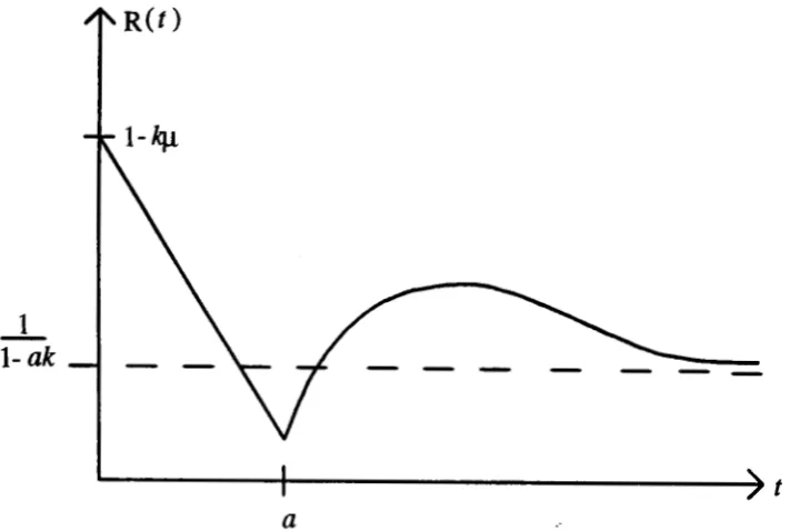
-18-Figure 2: Ske~ch of the Ruin function R(t).

The Ruin function R(t) is continuous Vt~ 0, differentiable Vt~ 0 \ {t =a} and approaches its limiting value 1

1-ak

From (21) a double pole occurs at s = 0 when 1-ak = 0, therefore

lim

{R(t)+~(l-kµ)t}

=

~(1-kµ).

~- a 3

4. ZEROS OF THE TRANSCENDENTAL EQUATION

Equation (4) is the transcendental equation associated with the differential-difference equation (1). The zeros of this equation are well documented and since many research papers have been interested in the stability of the solution of the differential-difference equation, conditions are given for the existence of complex conjugate roots with negative real part. From Bellman and Cooke [l] a necessary and sufficient condition for (4) to have roots with negative real part is

(i)

ab>

1.

(ii)

-ab<ac<~~

2

+(ab)

2

where~ istherootof~+abtan~=O 0<~<1t

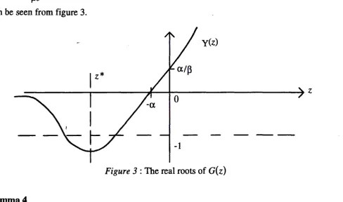
Lemma3

Equation ( 4) has at most 2 real zeros.

Proof: From (4), let z =as , a= ab , ~

=

ac , a> 0 , g(as)

=

G(z)

and so

G(z)

= z+a+~e-z =0 ₍₂₂₎

1

Let

Y(z)

=

13(z+a)ez

= -1 then at the turning point

z*

= -(l+a.),

Y(z*}

= -

~)+a.

Hence, since

l~et+ul

< 1, if

Y

{z*}<-1 there exists at most 2 real roots as

can be seen from figure 3.

y(z)

0

-1

Figure 3 : The real roots of

G(z)

Lemma4

Equation (22) has a.finite number of complex roots with positive real part.

Proof. Let

z

=

x+iy , then from (22)

x+a+~e-xCosy =

O}

y-~e-xSiny = 0 (23)

The zeros of

G(z)

depend continuously on ~ , and for ~ > 0 all zeros will be in the half plane

Re (z) =::;; ~· If G(z) = G' (z) = 0 there will be a double root at z + 1+a=0 and therefore

Utilizing similar arguments to that of Cooke and Grossman [8] it can be seen that if z = z(~)

is an isolated simple zero with Re (z) ~ 0, then it moves to the right of the half plane for increasing

p ,

since

and

dz

d~ =

Re(:)

=

dGI dP z+a

=

-dG/dz ~(l+z+a)

(x+a)(x+a+ 1)+

y2

(x+l+a)2+y2

> 0.

Suppose a pure imaginary root exists, then z = iy and a manipulation of (23) results in

y2

= ~1

-a2

For P increasing from a to oo these exists an increasing sequence

with

Sin~p

2 - a2 > O

such that for Pe(pk(a), Pk+i (a)) equation (22) has precisely k complex roots with positive real part. Also, whenever P =Pk (a) there exists a pair of complex conjugate imaginary roots

±

i Yk such that

7t

( 4k

+

1) - < Yk < (2k

+

1)7t , k

=

0, 1, 2, 3,. ... 2

It appears from (23) that a zero must remain in the region where Siny>O and Cosy< 0.

In the specific case where a

=

0 then

7t

P=Yk

=

(4k+l)- k=O, 1, 2, 3, ... .

'

5. NUMERICAL EXAMPLES

The roots of the characteristic equation can be located using

Mathematica.

Let

s

=

x+iy

then

R(x,y)=O

I(x,y)=O

s+b+ce-as=O

=

x+b+ce-axCosay

=

y-ce-axSinay.

(24)

Note that in (24) if for any

x,

y is a solution then so is -y. Hence the non-real zeros occur in

complex conjugate pairs.

Putting t = - a't, then (10) can be restated as

oo ("'+ )" -at(b+~1} ( ) " (

)r( )

L

(aceab)"

~

n

=

e

=

e-akf,

~

:t

.£

.

;

('t+rt

n=O

n

! 1

+

ab

+

a~l n=O

n .

r=O

b

(25)

where ~

1

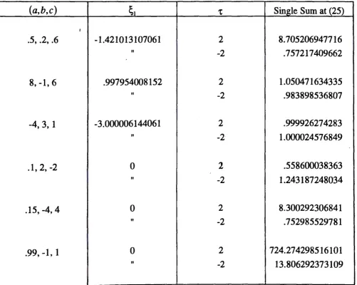
is the dominant root of the characteristic equation.

(a,b,c)

_~1

't Single Sum at (25)

I

.5, .2, .6 -1.421013107061 2 8.705206947716

II

-2 .757217409662

8, -1, 6 .997954008152 2 1.050471634335

II _{-2 .983898536807}

-4, 3, 1 -3.000006144061 2 .999926274283 '

II _{-2 1.000024576849}

.1,2,-2 0 2 .558600038363

II

-2 1.243187248034

.15,-4,4 0 2 8.300292306841

II _{-2 . 7 52985529781}

!

.99, -1, 1 0 2 724.274298516101

It

-2 13.806292373109

In table l, the single sum converges to the closed form term at (25) to within a truncation error Of E = 10-12•

Using the technique developed by Braden [4] the single positive sum needs at least 245 terms so that its sum is within a truncation error of e = 10-12 for (a, b, c) = ( .15, - 4, 4) and over one million terms for (a, b, c) = (. 99, - 1, 1) and t = 2 .

The double sum in (10), when it converges, generally requires many more terms in it's series

than does the single sum to converge to some prescribed truncation error. In Table 1 the double series converges only for the cases (a, b, c) = (.5, .2, .6) and (.1, 2, -2).

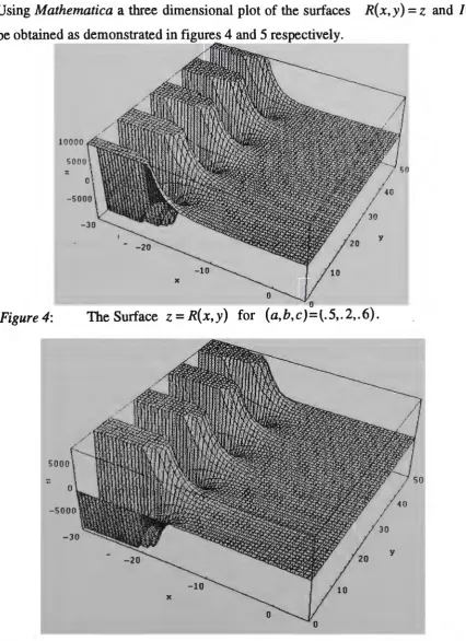
Using Mathematica a three dimensional plot of the surfaces

R(x,y)

= z and

I(x,y)

= z can

be obtained as demonstrated in figures 4 and 5 respectively.

10000

5000

z

y

x

0

Figure 4:

01

-The Surface

z

=

R(x,y}

for (a,b,c)=t.5,.2,.6).

CONCLUSION

A technique has been demonstrated whereby series may be represented in closed form. An

association was made between a differential-difference equation and its characteristic

equation, however a starting point may simply be taken as a Laplace transform equation of the

type

F(s)=---1

-P,,

(s

)+

Qn (s

)e-as

for Pn

(s)

and Qn

(s)

polynomials in

s

.

· In a follow up paper more general systems of the type

~

(:}-o'

t<»(1)-

f(t-a)

=

c(t)

and

f

(R)(-It

iR-k)(t-ka)

=

h(t)

k=O k

will be considered, together with equations that have more than one delay and equations of

neutral and mixed types.

Acknowledgments

The initial inspiration leading to this work was provided to the first named author by the late

Professor A. Keane. The authors also wish to acknowledge the helpful discussions with

REFERENCES

1. R. Bellman and K.L. Cooke. Differential-Difference Equations, Academic Press,

New York, London, 1963.

2. D.M. Bloom. Advanced Problein 6652, American Mathematical Monthly, 98 (1991), 272-3.

3. J.M. Borwein and P. B. Borwein. Strange Series and High Precision Fraud,

American Mathematical Monthly, 99 (1992), 622-640.

4. B. Braden. Calculating Sums of Infinite Series, American Mathematical Monthly, 99 (1992), 649-655.

5. F. Brauer: Absolute Stability in Delay Equations, Journal of Differential Equations,

69 (1987), 185-191.

6. F. Brauer and M. Zhien. Stability of Stage-Structured Population Models, Journal of

Mathematical Analysis and Applications, 126 (1987), 301-315.

7. R. K. Brayton. Bifurcation of Periodic Solutions in a Nonlinear

Difference-Differential Equation of Neutral Type, Quarterly of Applied Mathematics, 24 (1966),

215-224.

8. K. L. Cooke and Z. Grossman. Discrete Delay, Distributed Delay and Stability

Switches, Journal of Mathematical Analysis and Applications, 86 (1982), 592-627.

9. K. L. Cooke and P. van den Driessche. On Zeros of Some Transcendental Equations,

Funkcialaj Ekvacioj, 29 (1986), 77-90.

10. R. D. Driver, D. W. Sasser and M. L. Slater. The equation x' (t)=ax(t)+bx(t-'t)

with "Small" Delay, American Mathematical Society, 80 (1973), 990-995.

11. E. Brockmeyer and H. L. Halstrom. The Life and Works of A. K Erlang, Copenhagen

1948.

12.

w.

Feller. An Introduction to Probability Theory and its Applications, John Wiley

13. M. K. Grammatikopoulos and I. P. Stravroulakis. Necessary and Sufficient

Conditions for Oscillation of Neutral Equations with Deviating Arguments J. London Math. Soc., (2) 41 (1990), 244-260.

14. J. K. Hale. Homoclinic Orbits and Chaos in Delay Equations, Pitman Research Lecture Notes 157 (1987), 75-94.

15. J. K. Hale and S. M. Yerduyn Lunel. Introduction to Functional Differential Equations, Springer Verlag, New York 1993.

16. D. Y. Hao and F. Brauer. Analysis of a characteristic Equation, Journal of Integral Equations and Applications, 3 (1991), 239-253.

17. R. Holzsager. Solution to Asymptotic Linearity. American Mathematical Monthly, 99 (1992), 878-880.

18. A. Keane. Slowing Down from an Energy Distributed Neutron Source, Nuclear

Science and Engineering, 10 (1961), 117-119.

19. N. Minorsky,. Nonlinear Oscillations, D. Van Nostrand Company, Inc., Princeton

1962.

20. A. Pages and M. Gondran. System Reliability Evaluation and Prediction in

Engineering, North Oxford Academic 1986.

21. L. S. Pontryagin. On the zeros of Some Elementary Transcendental Functions,

American Mathematical Soc. Trans., Series 2, 1 (1955), 95-110.

22. G. Seifert. On an Interval Map Associated with a Delay Logistic Equation with

Discontinuous Delays, Lecture Notes in Mathematics, 1475 (1991), 243-249.

23. T. Teichmann. Slowing Down of Neutrons, Nuclear Science and Engineering,

7 (1960), 292-294.

24. H. C. Tijms. Stochastic Modelling and Analysis : A Computational Approach,

John Wiley and Sons, Chichester, 1986.

-26-26. E.T. Whittaker and G. N. Watson. A Course of Modern Analysis, Cambridge

University Press, Cambridge, Fourth Edition, reprinted 1978.

27. W.M.C. problem group. Solution to Asymptotic Linearity. American Mathematical

Monthly, 99 (1992), 877-878.

28. E. M. Wright. Stability Criteria and the Real Roots of a Transcendental Equation,