Semantically Secure Order-Revealing Encryption: Multi-Input Functional Encryption Without Obfuscation

Semantically Secure Order-Revealing Encryption:

Multi-Input Functional Encryption Without Obfuscation

Dan Boneh1_{, Kevin Lewi}1_{, Mariana Raykova}2_{, Amit Sahai}3_{, Mark Zhandry}1_{, and Joe Zimmerman}1

1_{Stanford University} 2_SRI

3_{Computer Science, UCLA and Center for Encrypted Functionalities}

Abstract

Deciding “greater-than” relations among data items just given their encryptions is at the heart of search algorithms on encrypted data, most notably, non-interactive binary search on encrypted data. Order-preserving encryption provides one solution, but provably provides only limited security guarantees. Two-input functional encryption is another approach, but requires the full power of obfuscation machinery and is currently not implementable.

We construct the first implementable encryption system supporting greater-than comparisons on encrypted data that provides the “best-possible” semantic security. In our scheme there is a public algorithm that given two ciphertexts as input, reveals the order of the corresponding plaintexts and nothing else. Our constructions are inspired by obfuscation techniques, but do not use obfuscation. For example, to compare two 16-bit encrypted values (e.g., salaries or age) we only need a 9-way multilinear map. More generally, comparingk-bit values requires only a(k/2 + 1)-way multilinear map. The required degree of multilinearity can be further reduced, but at the cost of increasing ciphertext size.

Beyond comparisons, our results give an implementable secret-key multi-input functional encryption scheme for functionalities that can be expressed as (generalized) branching programs of polynomial length and width. Comparisons are a special case of this class, where fork-bit inputs the branching program is of lengthk+ 1and width4.

1

Introduction

Functional encryption [BSW11] is a public-key encryption system that supports “partial” decryption keys: decrypting a ciphertextc=E(pk, m)using a keyskf revealsf(m)and nothing else. Multi-input functional

encryption [GGG+14] is a generalization of functional encryption where the keyskf acts on`ciphertexts

c1 =E(pk, m1), . . . , c` =E(pk, m`)to revealf(m1, . . . , m`)and nothing else. Existing constructions for

general multi-input functional encryption are based on obfuscation and thus are not currently feasible to implement, even for simple functionalities.

In this paper we present a construction forsecret-keymulti-input functional encryption from multilinear maps. By restricting our attention to the secret-key setting, we are able to achieve a much more efficient construction, without the full machinery of obfuscation and NIZK proofs.

1.1 Order-revealing encryption

Definition. A secret-key encryption scheme isorder-revealing1[BCO11] if there is a public procedure that takes twoencryptedplaintexts as input and reports their lexicographic ordering. This procedure, which we call the order-revealing algorithm, requires no secrets and can be evaluated by anyone. More precisely, an order-revealing scheme is a tuple(G, E, D)of algorithms. AlgorithmGoutputs a pair(sk,comp)wheresk

is a secret encryption key andcomp(·,·)is an efficient deterministic algorithm that takes two ciphertexts as input and outputs either ‘<’ or ‘≥’. AlgorithmsE(sk, m)andD(sk, c)are standard encryption/decryption algorithms wherem∈ {0, . . . , B}for someB. In addition to the standard correctness of decryption we also require that for all(sk,comp)output byGand for all plaintextsm0, m1we have:

m0< m1 =⇒ Pr[comp(E(sk, m0), E(sk, m1) ) =0<0] = 1

m0≥m1 =⇒ Pr[comp(E(sk, m0), E(sk, m1) ) =0≥0] = 1

An order-revealing encryption scheme is secure if a ciphertext reveals nothing about the corresponding plaintext beyond its lexicographic relation relative to other ciphertexts. This is defined using a simple variant of the standard semantic security game [GM82]: the adversary is given algorithmcomp(·,·)and access to a “left-right-oracle”O(·,·)that on input(m0, m1)returnsE(sk, mb)for someb∈ {0,1}chosen at the

beginning of the game. After adaptively querying the oracleOthe adversary outputs a guessb0 and wins the game ifb=b0. Let(m(0)₀ , m(0)₁ ), . . . ,(m(₀q), m(₁q))be the adversary’s queries toO. To ensure that the adversary cannot use algorithmcomp(·,·)to trivially win the game we require that the relative ordering of messages on the left is the same as the relative ordering on the right, namely for all0≤i, j≤q:

m(₀i)< m(₀j) ⇐⇒ m(₁i)< m(₁j)

The scheme is secure if the adversary cannot win this game with non-negligible advantage. We refer to this notion asbest-possible semantic security. We give a complete (and more general) definition in Section 4.

Note that apublic-keyorder-revealing encryption scheme is impossible: if an adversary has unrestricted access to the encryption algorithm, he can use the encryption algorithm and the order-revealing algorithm

comp(·,·)to decrypt any ciphertext using binary search without the secret key.

Applications. Order-revealing encryption (ORE) is motivated by the problem of answering range queries on a remote encrypted database [AKSX04, BCLO09]. Consider a remote database holding encrypted pairs

(name,salary). The data owner wishes to retrieve all records with a salary greater thant. If salaries are encrypted using an ORE then the database can sort all records on its own from lowest salary to highest. This sorting can be done even when records are inserted sequentially into the database (perhaps by multiple users who share the secret encryption key) and requires no interaction with the data owner(s). To issue the range query the data owner sends the encryption oftunder the ORE key. In response, the database first uses binary search on the encrypted salaries to locate the smallest encrypted recordRwith a salary greater thentand then simply sends all records to the “right” ofRback to the user. Thus, for a database ofnrecords, the database’s work isO(logn)and requires only one round of interaction with the client, as in the case of a cleartext database. Security of the ORE ensures that the database learns nothing beyond the relative ordering of records and queries.

1

Alternate approaches. Before describing our construction we briefly survey a few alternate constructions for answering range queries on a remote encrypted database.

Boldyreva et al. [BCLO09, BCO11] describe an elegant primitive called Order Preserving Encryption (OPE) where encryption preserves the relative ordering of plaintexts. Comparing encrypted data is then done by simply comparing the corresponding ciphertexts. However, OPE leaks information about the relative distances of plaintexts. Recent work of Malkin et al. [MTY13] constructs an OPE scheme with a partial security guarantee, hiding the low-order bits of plaintexts, but still does not achieve best-possible semantic security. Indeed, Boldyreva et al. [BCLO09] prove that no OPE scheme can possibly achieve best-possible semantic security. In ORE, unlike OPE, comparisons are done with a dedicated algorithmcomp(·,·)which is the reason best-possible semantic security can be achieved.

A very different approach to answering range queries on encrypted data uses garbled RAMs [LO13, GHL+14]. With garbled RAMs the database can answer range queries without learning any information about the data, but answering the range queries requires more rounds of interaction per query and the database’s work is higher than with ORE.

Other approaches to answering range queries are based on public-key predicate encryption [BW07, SBC+07, KSW08] and require a linear scan through the database. With ORE, range queries can be answered in logarithmic time in the size of the database. We also mention a result of Popa et al. [PLZ13] who describe an interactive protocol for answering range queries. Interaction is used to maintain a sorted data structure at the database by offloading some comparisons to the client. Finally, we note that ORE is a special case of secret-key two-input functional encryption [GGG+14].

1.2 Order revealing encryption: our construction

Our construction begins with a simple automaton for the comparison function on two inputs that we represent as a low-width matrix branching program. We encrypt ciphertexts in a way such that given two independently-created ciphertexts, anyone can run the comparison branching program to reveal the relative ordering of the corresponding plaintexts. While our encryption scheme applies to any multi-input functionality expressed as a matrix branching program (see Section 2.2), for the rest of this section we use the two-input comparison automaton and its branching program as a concrete example to illustrate the construction.

The comparison automaton and branching program. Figure 1 shows a five-state automaton A that computes the ordering of two inputsx = x1x2· · ·xn andy = y1y2. . . ynin {0,1}n when the input is

processed in an interleaved order (of the formx1y1x2y2· · ·xnyn). From this automaton we derive four 5×5matricesX0,X1,Y0,Y1, where each is the adjacency matrix of a subgraph ofA: forb∈ {0,1}, the

matrixXb is the adjacency matrix of the subgraph consisting only of theb-transitions used by input bits of

x, and the matrixYb is the adjacency matrix of the subgraph consisting only of theb-transitions used by

input bits ofy. Note that these matrices are not invertible because of the sink states in the automaton. This introduces additional challenges in the security proof; however, we are able to handle branching programs with non-invertible matrices using recent results of Sahai and Zhandry [SZ14].

Leteibe the 5-vector containing1in positioniand zero elsewhere. Then the producte|1·

Qn

i=1(XxiYyi)

results in a vector with a single “1” in three possible locations (corresponding to either the “x > y”, “x < y”, or “=” final states), and the location of the “1” determines the result of the comparison operation onxandy. Hence, the matricesX0,X1,Y0,Y1form a matrix branching program for the two-input comparison function.

In Section 3 we show that a simple re-ordering of the inputs reduces the matrix program length to onlyn+ 1

x>y$ x<y$ yi=1$

0

=$

1

y_i=1$ y_i=0$

0,1$ 0,1$

Figure 1: The5-state comparison automaton on inputsx, y∈ {0,1}n_{where ‘=’ is the start}

state. Input bits are processed in an interleaved orderx1y1x2y2. . .

A1# _D

1# A2# D2# A3# D3#

c_x#=#E(sk,##x₁#x₂#x₃)#

c_y#=#E(sk,##y₁#y₂#y₃)#

⟶

###z#

Figure 2: The order-revealing algorithm applied to encryptions ofx1x2x3 andy1y2y3.

The ORE encryption scheme. Fix a primeq. The setup algorithmGuniformly samples2n−1invertible matricesR1, . . . ,R2n−1fromGL5(Zq). These matrices form the secret encryption keysk. During encryption these matrices will be used to randomize the matrices of the comparison branching program using Kilian’s randomization technique [Kil88]. We define two additional vectorsR0:=e|1andR2n:=e5. The secret key

also contains the parameters for an asymmetric multilinear map [GGH13a] with2nindices (i.e., of degree

2n). We divide the2nindices into two disjoint size-nsetsU₁andU₂.

The encryption algorithm encrypts a plaintextx = x1x2· · ·xn ∈ {0,1}nas follows. It first samples

a partition(S1, . . . , Sn)ofU1and a partition(T1, . . . , Tn)ofU2. These partitions are sampled at random

from a family of partitions we call an “exclusive partition family.” They must satisfy a specific combinatorial property needed to prevent certain “mix-and-match” attacks where the attacker tries to run the comparison algorithm on improperly formed ciphertexts. We define and construct these partition families in Section 2.5. They are a generalization of the “straddling sets” used in Barak et al. [BGK+14].

Next, the encryption algorithm samples random scalarsα1, . . . , α2n ∈ Z∗q and constructs the 5×5

matrices

ˆ

Xi =αi·(R2i−2Xxi R −1

2i−1) and Yˆi =αn+i·(R2i−1YxiR −1 2i )

fori∈[n]where we defineR−_2n1 :=e5. Recall that the matricesRi are taken from the secret key and the

matricesX0,X1andY0,Y1are the matrices in the comparison branching program. BecauseR0andR2n

are vectors, so areXˆ0andYˆn. All other ciphertext components are square matrices.

Finally, for i ∈ [n]the encryption algorithm encodes the entries ofXˆi under the index setSi of the

multilinear map, and encodes the entries ofYˆi under the index setTi. The resulting2nencoded5×5

matrices({Xˆi}ni=1,{Yˆj}nj=1)are output as the encryption ofx∈ {0,1}n.

The order-revealing algorithm. Given two independently-created ciphertextscx andcy corresponding

to plaintextsxandy, the order-revealing algorithm computes the interleaved product of the matrices in the left half ofcx with the matrices in the right half ofcy. In other words, ifcx = ({Ai}ni=1,{Bj}nj=1)and

multilinear map and the result is a single group element (a scalar) becauseA1andDnare vectors. Finally,

the algorithm zero-testszand the outcome reveals the ordering ofxandy. Zero-testing thiszis possible because it is an encoding of an element under the full2nindex set, by the structure of the partitions.

To verify that the final zero-test correctly reveals the ordering ofxandy, observe that the scalarzexpands to the quantity

e|₁Xx1R −1 1

R1Yy1R −1 2

· · · R2n−2XxnR −1 2n−1

(R2n−1Yyne5) (1.1)

Hence,ztakes on a non-zero value if and only if the comparison automaton terminates in the state “x < y”. Note that we omitted the scalarsαi in the expansion (1.1) for ease of exposition. Their presence causeszto

be either0or non-zero, as opposed to0or1.

Security. We prove the security of a generalization of this construction in the generic multilinear map model [GGH+13b, BR14, BGK+14]. The use of Kilian’s randomization technique in the encryption key restricts the adversary’s ability to manipulate ciphertext components in an elementary manner, such as by computing products of matrices out of order. Also, the use of the random scalarsα1, . . . , α2nprevents the

adversary from correlating multiple encryptions of plaintexts which share the same bit pattern. However, there is still a large domain of attacks that the adversary could potentially take advantage of. For example, an adversary can combine components from multiple ciphertexts to look for relations, or he can compare the results of partial evaluations of the branching program on different inputs.

In order to handle these types of attacks, we use the combinatorial structure provided by our exclusive partition families. Intuitively, the use of a random partition from an exclusive partition family for each ciphertext ensures that if the adversary computes a partial evaluation of the branching program, or tries to mix components from multiple ciphertexts, he will not be able to obtain a group element which is encoded in the index set for the zero-tester, as required by the generic multilinear map model. In fact, it turns out that the use of these exclusive partition families is indeed sufficient to prove security of the construction in the generic model.

Performance. Our basic construction requires a(2n+ 2)-way multilinear map to evaluate comparisons onn-bit numbers. However, simple optimizations, including re-ordering of the matrices in the branching program, enables us to shrink the total length of the comparison branching program to only(n+ 1)matrices each of dimension4×4(see Section 2.2 for details). Consequently, we only need an(n+ 1)-way multilinear map to evaluate comparisons onn-bit numbers. The secret encryption key contains16nelements inZq,

and each ciphertext is16n−8encoded group elements. We can further reduce the required degree of multilinearity by a factor oflog₂Bby representing messages in base-B (instead of base-2) and modifying the comparison automaton to compare one base-B digit per step. This shortens the length of the branching program (and therefore the degree of multilinearity) by a factor of log₂B, but at the cost of increasing the number of states in the automaton by a factor ofB and consequently increasing the number of group elements in the ciphertext by a factor of approximatelyB2/log₂B. For example, moving to baseB = 4

gives multilinearity(n/2 + 1), with ciphertexts requiring18n−24group elements.

Generalizing to multi-input functional encryption. While we used order-revealing encryption (ORE) as an example application, our construction is more general: it gives a secret-key multi-input functional encryption where the degree of multilinearity needed for decrypting with a keyskf depends on the length of

the branching program representingf. In fact, every matrix in the branching program can depend onallthe bits of one of the inputs tof and this can be used to shrink the length of the branching program. We refer to these asgeneralized branching programsand define them precisely in the next section.

Our base multi-input functional encryption scheme supports a single functionf (such as comparison) fixed a-priori during initial key generation. This functionf defines the branching program relative to which all encryptions are computed. This apparent single-function limitation is easily removed using universal circuits: the functionality fixed a-priori is a universal circuitUthat takes as input the description of a function f and its inputsx1, . . . , xnand outputsf(x1, . . . , xn). Now, a functional encryption “key”skf for a function

f is simply the encryption off under our encryption scheme. Givenskf and the encryptions ofx1, . . . , xn

the functionality for the universal circuitUcan be used to computef(x1, . . . , xn)in the clear.

1.3 Other related work

Multi-input functional encryption was introduced by Goldwasser et al. [GGG+14], who gave constructions based on indistinguishability obfuscation [BGI+01, GGH+13b] and differing-inputs obfuscation [BGI+01, BCP14, ABG+13].

Our construction of multi-input functional encryption is inspired by obfuscation techniques [GGH+13b, BBC+14, AGIS14], but does not use obfuscation. Instead we build multi-input functional encryption directly from multilinear maps. Several other results use obfuscation techniques to obtain more efficient constructions directly from multilinear maps. Zhandry [Zha14] showed how to constructn-way Diffie-Hellman key ex-change without trusted setup, a result that was previously known only using obfuscation [BZ14]. Concurrently with this work, Garg et al. [GGHZ14] showed how to construct single-input functional encryption from multilinear maps; however, their motivation was to obtain security proofs from concrete assumptions, rather than efficiency. The constructions in this paper are considerably more efficient (we make use of a much smaller number of matrices), but our security proof is in the generic multilinear map model.

Single-input functional encryption [BSW11] has been traditionally defined in the public-key settings and studied extensively [O’N10, GVW12, AGVW13, BO13, CIJ+13, GGH+13b, GKP+13, BCP14]. In this paper, however, we focus on secret-key (multi-input) functional encryption, which is sufficient for data processing on a remote encrypted database, including order-revealing encryption. Focusing on the secret-key setting enables us to give a simple construction from multilinear maps. Single-inputsecret-keyfunctional encryption was previously explored for the inner-product functionality by Shen et al. [SSW09] and more generally by Goldwasser et al. [GKP+13]. Brakerski and Segev [BS14] recently showed how to convert any secret-key functional encryption scheme into one where secret keys do not reveal their functionality.

2

Preliminaries

2.1 Conventions

For an integern, we write[n]to denote the set{1, . . . , n}. For a finite setS, we writeUniform(S)to denote the probability distribution that is uniform over the elements ofS. When working with vectors inZnfor some integern, for eachi∈[n]we writeeito denote theithunit column vector, i.e., the vector(x1, x2, . . . , xn)|

2.2 Matrix Branching Programs (MBPs)

In this section, we define a variant of matrix branching programs for which our main construction applies. These generalized matrix branching programs are a sequence of efficiently computable Boolean circuits that turn a given multi-variate input into a matrix.

Definition 2.1(Generalized Matrix Branching Program). LetX ⊂ {0,1}∗be a set of possible input strings, and letf :Xm_{→ {0,1}be a multi-input function. Ageneralized matrix branching programP of length`}

and widthw, overZqfor a primeq, is a tuple of the form

P = (q, m, d, inp, (M₁, . . . , M_`) ),

where for eachj∈[`], the functionM_j :X →_Zw×w_q is computable by an efficient deterministic algorithm. The valueinpis a lookup table of the form

inp= (inp(1), . . . , inp(`)),

where for eachj ∈[`], we haveinp(j)∈ [m]. The branching program takesminputs and we say that at stepjitinspectsinput numberinp(j) ∈ [m]. To simplify notation, we require the branching program to inspect each of itsminput variables exactlydtimes2(so that the length of the program,`, is preciselymd). We also introduce the following shorthand notations:

• For a branching program stepj∈[`], input sloti∈[m], and sub-indexh∈[d], we writej=inp.j(i, h)

to signify thatjis the step in which the program inspects input slotifor thehthtime.

• For a branching program stepj∈[`]and sub-indexh∈[d], we writeh=inp.h(j)to signify thatjis the step in which the program inspects the corresponding input slotinp(j)for thehthtime.

We say thatP computesthe functionf if, for all inputsx= (x(1), . . . , x(m))∈ Xm_,



 Y

j∈[`]

M_j(x(inp(j)))



[1,1] = 0 ⇐⇒ f(x) = 1.

Since every programP computes a unique functionf, we also writeP(x)to denotef(x).

Following Sahai and Zhandry [SZ14], we also define the notion of anon-shortcuttingmatrix branching program.

Definition 2.2(Shortcuts in Matrix Branching Programs [SZ14]). A branching program has ashortcuton inputx= (x(1), . . . , x(m))∈ Xm_{if either:}



 Y

j∈[`]

Mj(x(inp(j)))



·e1 =0w×1 or e|1·



 Y

j∈[`]

Mj(x(inp(j)))



=01×w

2

In such a case, it is possible to determine thatf(x) = 1without carrying out the entire matrix product. We say that a branching program isnon-shortcuttingif, for all inputsx, it has no shortcuts onx. We require that every generalized matrix branching program is non-shortcutting.

We note that there are multiple ways to obtain a generalized matrix branching program from a circuit, or from a time-bounded Turing machine or RAM. Barrington’s theorem [Bar86] shows how to convert a Boolean circuit of depthdinto a matrix branching program of lengthO(4d)and width5. The work of Ananth, Gupta, Ishai, and Sahai [AGIS14] takes a different approach to obtain MBPs for Boolean formulas that avoids the complexity of Barrington’s construction. They construct a layered automaton for any Boolean formula which consists of several states including a starting state and an accepting state together with edges denoting the transitions between states based on the input bit values. Given such an automaton representation, a formula can be evaluated by counting the number of paths between the starting and the accepting state. Ananth et al. show that a Boolean formula of sizescan be converted into a layered graph-based branching program with O(s)layers with matrices of sizeO(s2). Thus, the size of the resulting MBP isO(s3). Subsequently, Sahai and Zhandry [SZ14] improve the conversion, giving MBP’s of lengthO(s)and sizeO(s(log₂s)2). Our approach follows the general method of computing automata with generalized MBPs, but we observe that for some problems such as comparing two-bit strings, we can directly construct extremely efficient automata that do not use the general translation from formulas to automata.

For more details, we refer the reader to Section 3.

2.3 Randomized Matrix Branching Programs

In our construction, as in obfuscation constructions that use MBPs [GGH+13b, BGK+14, BR14, AGIS14], we must make sure that the adversary always evaluates the MBP by multiplying together one matrix selection for each stepj∈[`]. In particular, we must ensure that partial matrix products, which omit some steps, will not reveal any information about the program.

The main ingredient we need here is the MBP randomization technique of Kilian [Kil88], in which we pre-and post-multiply each matrix in the MBP by matching, invertible rpre-andom “blinding” matricesR0, . . . ,R`.

Intuitively, the resulting randomized MBP fixes the order in which the randomized MBP matrices can be multiplied, i.e., requiring one matrix for each step in the original MBP. Any other product will also contain at least one random “blinding” matrix, rendering the result useless to the adversary.

In addition, we combine Kilian’s randomization technique with “bookend vectors”ˆs,ˆt, as introduced in [GGH+13b], which further restrict the adversary to projecting a single scalar entry of the matrix product resulting from the MBP evaluation (namely, the entry at position[1,1]). Testing whether this scalar is zero suffices to determine the Boolean output of the program, while preventing the adversary from learning extra information by testing other matrix entries.

We now present the details of the randomized MBP construction.

Definition 2.3 (Randomized MBPs ([Kil88], adapted)). We define an efficient randomized procedure

MBPRand, such that, for a given generalized matrix branching program

P = (q, m, d, inp, (M₁, . . . , M_`) ),

the procedureMBPRand(P)outputs a tuplePˆ of the form

ˆ

P =

q, m, d, inp, ( ˆM1, . . . , Mˆ`), ˆs, ˆt

where, for eachj∈[`], the functionMˆ_j :X →_Zw×w

q is represented, likeMj, as a Boolean circuit; andˆs

andˆtare vectors inZwq.

The procedureMBPRandoperates as follows. It samples(`+1)invertible matricesR0, . . . ,R`uniformly

at random fromGLw(Zq). It computes the values

ˆs=e|₁R₀−1 and ˆt=R`e1,

and, for eachj∈[`], the functionMˆ_j defined as

ˆ

M_j(x) =R−_j−1₁M_j(x)Rj.

Finally, it outputs the tuple

ˆ

P =q, m, d, inp, ( ˆM1, . . . , Mˆ`), ˆs, ˆt

.

To evaluate a randomized MBPPˆ on an inputx = (x(1), . . . , x(m)), we run each (randomized) ma-trix functionMˆj on the indicated input string x(inp(j)), producing a randomized matrix Mj. We write MBPSelect( ˆP ,x)to denote the sequence of randomized matrices and bookend vectors (ˆs,M1, . . . ,M`,ˆt),

and to evaluate the program, we multiply all of these randomized matrices and vectors together. Formally, we define the following procedures.

Definition 2.4(Evaluation for Randomized MBPs ([Kil88], adapted)). Fix a generalized matrix branching programPand a vector of inputsx= (x(1), . . . , x(m))∈ Xm_{, and suppose that}

ˆ

P =q, m, d, inp, ( ˆM₁, . . . , Mˆ_`), ˆs, ˆt ← MBPRand(P).

For eachj∈[`], we defineMˆj = ˆMj(x(inp(j))), and we define

MBPSelect( ˆP ,x) =

ˆs|, Mˆ1, . . . ,Mˆ`, ˆt

.

Finally, we define

MBPEvalˆs|, Mˆ1, . . . ,Mˆ`, ˆt

= ˆs|



 Y

j∈` ˆ

Mj



ˆt.

Given the above definitions, the proof of the following lemma follows immediately.

Lemma 2.5(Correctness for Randomized MBPs). Fix a generalized matrix branching programP, and a vector of inputsx= (x(1), . . . , x(m))∈ Xm_{. Then,}

MBPEval(MBPSelect( ˆP ,x)) = 0 ⇐⇒ f(x) = 1.

Ordinarily, for MBPs derived from Barrington’s theorem [Bar86], we would also be able to state a simulation theorem, showing that the output distribution MBPSelect( ˆP ,x) depends only the output of the original program, P(x). In our construction, however, we obtain much more efficient programs by other techniques (Section 3), and the matrices Mj(x) in these programs do not always have full rank.

Indeed, the kernel of each matrix may depend on the input vectorx, and as a result, the output distributions

MBPSelect( ˆP ,·)may be noticeably different for different inputsx0,x1, even if the outputs of the program,

Instead of constructing a simulator, we rely on a weaker property that is still strong enough to prove secu-rity of our main construction. Specifically, we show that even though the distributionsMBPSelect( ˆP ,x0)and

MBPSelect( ˆP ,x1)may differ, they cannot be distinguished by a certain weak family of tests; in our

construc-tion (Secconstruc-tion 5), we will show that these are the only tests an adversary can possibly perform in our security model. To define such a family of tests, we refer to the following definition of Sahai and Zhandry [SZ14].

Definition 2.6(Allowable Tests [SZ14]). Letp:Z2w+w

2_`

q →Zqbe a multilinear (multivariate) polynomial

over the entries ofˆs,ˆt∈Zwq andMˆ1, . . . ,Mˆ`∈Zw×wq (as formal variables). We saypis anallowabletest

polynomial if each monomial in the expansion ofpcontains at most one entry of each vectorˆs,ˆtand matrix

ˆ

M1, . . . ,Mˆ`.

Lemma 2.7(Security for Randomized MBPs). Fix a non-shortcutting generalized matrix branching program P(overZq, forq >2λ), two input vectorsx0,x1such thatP(x0) =P(x1), and an allowable test polynomial

p(Def. 2.6). Then either

PrhPˆ ←MBPRand(P) ; p(MBPSelect( ˆP ,xb)) = 0

i

= 1

for both bitsb∈ {0,1}, or,

PrhPˆ ←MBPRand(P) ; p(MBPSelect( ˆP ,xb)) = 0

i

<negl(λ)

for both bitsb∈ {0,1}.

Lemma 2.7 follows immediately from the results of Sahai and Zhandry [SZ14]; we defer the formal treatment to Appendix A.1.

2.4 Multilinear Maps

Multilinear maps [BS03], also known as graded encodings, or graded multilinear maps [GGH13a, CLT13], are a generalization of bilinear maps such as pairings over elliptic curves [Mil04, MOV93, Jou00, BF01]. Roughly speaking, a multilinear map lets us take a scalarx∈Fqand produce an encoded version,xˆ= [x]S,

whereS⊆ U is a finite set, called anindex set, that indicates the level of the encodingxˆin a given hierarchy (namely, the subsets ofU ordered by inclusion).3

By convention, we will say that these index sets are made up offormal symbols, denoted by capital letters (A, B, C), which serve the same role as formal variables in polynomials. To be fully precise, we state the following definitions.

Definition 2.8(Formal Symbol). Aformal symbolis a bit string in{0,1}∗_{, and distinct variables denote}

distinct bit strings. Afreshformal symbol is any bit string in{0,1}∗that has not already been assigned to another formal symbol.

Definition 2.9(Index Sets). An index setis a set of formal symbols calledindices. By convention, for index sets we use set notation and product notation interchangeably, so thatABC represents{A, B, C}, and

ABC∪D=ABCD.

Definition 2.10 (Multilinear Map ([BS03, GGH13a, CLT13])). A multilinear map over prime-order fi-nite fields supports the following operations. Each of the operations (MM.Setup, MM.Add, MM.Mult,

MM.ZeroTest,MM.Encode) is implemented by an efficient randomized algorithm.

3

• The setup procedure receives as input an index setU(Definition 2.9), which we refer to as the “top-level index set”, as well as the security parameterλ(in unary). It produces public parameterspp(which include anO(λ)-bit primeq), and secret evaluation parameterssk:

MM.Setup(U, 1λ) → (pp, sk)

• For each index setS ⊆ U, and each scalarx∈_Zq, there is a set of strings[x]S ⊆ {0,1}∗, i.e., the set

of all valid encodings ofxat index setS.4 From here on, we will abuse notation to write[x]S to stand for any element of[x]S(i.e., any valid encoding ofxat the index setS).

• Elements at the same index setS ⊆ U can be added, with the result also encoded atS:

MM.Add(pp, [x]S, [y]S) → [x+y]S

• Elements at two index setsS1,S2can be multiplied, with the result encoded at the union of the two

sets, as long as their union is still contained inU:

MM.Mult(pp, [x]S1, [y]S2) →

(

[xy]S1∪S2 ifS1∪ S2 ⊆ U

⊥ otherwise

• Elements at the top levelU can bezero-tested:

MM.ZeroTest(pp, [x]S) →

(

“zero” ifS =U andx= 0∈_Zq

“nonzero” otherwise

• Using the secret parameters, one can generate a representation of a given scalarx∈_Zqat any index

setS ⊆ U:

MM.Encode(sp, x, S) → [x]S

• For the trivial index setS =∅, we specify that the only valid encoding of[x]∅is just the scalarx∈Fq.

(So, for instance, we can perform subtraction viaMM.Add, by scalar multiplication with−1.)

By convention, we refer to the cardinality ofU as thedegree of multilinearityof the map.5 Technically, known instantiations of multilinear maps [GGH13a, CLT13] are only approximate, and have a “noise” term that restricts the degree of multilinearity to a pre-specified polynomial in the security parameter. However, this restriction will not affect our results in this work, and to keep the presentation simple we do not model the restriction formally.

When the context is clear, we also abuse notation to write, for encoded elementsa,ˆ ˆb, the expressionˆa+ ˆb to meanMM.Add(MM.pp,ˆa,ˆb); the expressionˆaˆbto meanMM.Mult(MM.pp,ˆa,ˆb); and likewise for other arithmetic expressions.

4_{To be more precise, we define[x]S={χ∈ {0,1}}∗

:MM.IsEncoding(pp, χ, x,S)}, where the predicateMM.IsEncodingis specified by the concrete instantiation of the multilinear map. In general, the predicateMM.IsEncodingis not necessarily efficiently decidable—and indeed, for the security of the multilinear map, it should not be.

5

The generic multilinear map model. To define security, we will operate in the generic multilinear map model (also known as thegeneric graded encoding model[GGH+13b, BR14, BGK+14]). This model is very similar to the generic group model [Sho97]—intuitively, in this model, the only operations an adversary can use with encoded elements are the operations of the multilinear map. More precisely, we say a scheme that uses multilinear maps is secure in the generic multilinear map model if, for any concrete adversary breaking the real scheme, there is an ideal adversary breaking a modified scheme in which each concrete encoded element is replaced by a “handle” (concretely, a fresh nonce), mapped to the actual encoded scalar in a table unavailable to the adversary. Each multilinear map operation is replaced by an oracle query that takes two handles and returns another fresh handle (creating a new table entry), except for the zero-test oracle query, which, when given a handle, returns “zero” if the corresponding scalar in the table is zero, and “nonzero” otherwise. We defer the formal definitions to Appendix C.

2.5 Exclusive Partition Families

Even though the randomized MBPs of Section 2.3 impose certain restrictions on how their matrices can be multiplied together to remove the randomizing factors, this alone does not prevent an adversary from learning more information than just the outputs of honest evaluations on the MBP. The issue is that the adversary may execute “mix-and-match” attacks, using encoded matrices from multiple ciphertexts in the same evaluation. Our construction will use the multilinear map’s index sets to enforce constraints on the adversary’s evaluation, ruling out this kind of attack. As with the “straddling sets” technique of Barak et al. [BGK+14], in order to use index sets to enforce this restriction, we need to design these index sets with some combinatorial properties in mind.

In more detail, suppose U is the top-level index set in the multilinear map, andF is some family of partitions ofU. Intuitively, whenever weintendterms to be multiplied together (e.g., because they are matrix elements from a consistent choice of ciphertexts), the index sets of those terms will partitionU, so that the product of the encoded elements can legally be zero-tested. We will design the partition familyFso that our intended partitions (those inF) are the only partitions ofU that the adversary can possibly construct given the index sets of the terms we provide, thereby ruling out “mix-and-match” attacks.

Formally, we define the following:

Definition 2.11(Partition). The collection of setsP ={S1, . . . , Sd}is apartitionof a setUifS1∪· · ·∪Sd=

U; eachSiis a nonempty subset ofU; andSi∩Sj =∅for eachi6=j.

Definition 2.12(Exclusive Partition Family). Fix a setU, and a familyF of partitions ofU, where we write theN partitions in the familyFas the rows of the matrix:



 

S1,1 S1,2 · · · S1,d

..

. ... . .. ... SN,1 SN,2 · · · SN,d



 

We say thatF is an(N,d)-exclusive partition familyofU if the only partitions ofU that can be formed from sets inFare precisely the rows of the matrix. (Formally: for all(i1, j1), . . . ,(im, jm)∈[N]×[d], the

collectionP ={S_i1,j1, . . . , Sim,jm}is a partition ofU if and only ifi1=. . .=imand{j1, . . . , jm}= [d].)

We say that an exclusive partition familyF isexplicitif there is an efficient deterministic algorithm which, when giveni∈[N], j∈[d], outputs the elements ofSi,j (i.e., outputs the index of each element in

partition(Si,1, . . . , Si,d)uniformly over all of the partitions inF, simply by choosing uniformi←[N]. To

simplify notation, we write this sampling procedure as(Si,1, . . . , Si,d)

$

← F.

Construction 2.13((2λ, d)-Exclusive Partition Families). Letd, λ >0be integers, and letU be a set of size

(1 + (d−1)(λ+ 1)). Denote the elements ofU as

U ={a1, a2, . . . , ad, b2,1, . . . , b2,λ, . . . , bd,1, . . . , bd,λ},

and identify an indexi∈[2λ]with the stringρ(i)∈ {0,1}λ_{that forms the binary representation of(i−1).}

Define

Si,1={a1} ∪

[

j∈{2,...,d}

{bj,k :ρ(i)k = 1}

and for eachj∈ {2, . . . , d}, define

Si,j ={aj} ∪ {bj,k :ρ(i)k= 0}.

Finally, define the familyF(d, λ) = ((S1,1, . . . , S1,d), . . . ,(SN,1, . . . , SN,d)).

Lemma 2.14((2λ, d)-Exclusive Partition Families). For integersd, λ > 0, the familyF(d, λ)defined by Construction 2.13 is an explicit(2λ, d)-exclusive partition family.

Proof. By construction, each(Si,1, . . . , Si,d)is a partition ofU consisting ofdsets, and the elements of each

set are efficiently computable. Now, suppose that for some choice of sets(i1, j1), . . . ,(im, jm)∈[N]×[d],

the collectionP ={Si1,j1, . . . , Sim,jm}is a partition ofU. Then there exists somer

∗ _{∈[m]such that the}

setSir∗,jr∗ containsa1. The only such sets are of the form:

Sir∗,jr∗ =Sir∗,1={a1} ∪

[

j∈{2,...,d}

{b_j,k :ρ(ir∗)_k= 1}

Assume for sake of contradiction that for somer∈[m],ir 6=ir∗. We cannot havej_r= 1, since this would cover the elementa1twice: once bySir∗,jr∗, and once bySir,jr. Thusjr∈ {2, . . . , d}, and the setSir,jr is

of the form:

Sir,jr ={ajr} ∪ {bjr,k :ρ(ir)k = 0}

But for eachk ∈ [λ], the only sets that containbjr,k also contain eithera1 orajr, and we already have

a1 ∈ Si∗_,1 anda_j

r ∈ Sir,jr covered by the putative partitionP. Hence the only elementsbjr,k that are

covered byP are those of the form{b_j,k : ρ(ir∗)_k = 1} and{b_j,k : ρ(i_r)_k = 0}. Since by assumption ir6=ir∗, the stringsρ(ir), ρ(i_r∗)differ on some bitk∗ ∈[λ]. Ifρ(i_r∗)k∗ = 0andρ(ir)k = 1, thenP fails to coverbjr,k∗, while ifρ(ir∗)k∗ = 1andρ(ir)k = 0, thenP coversbjr,k∗twice. In either caseP is not a

partition ofU, contradicting our assumption. So we conclude thatir∗ =i₁ =. . .=i_m, and thusF is an explicit(2λ, d)-exclusive partition family.

We also observe that our definition of exclusive partition families generalizes thestraddling set systemsof Barak et al. [BGK+14]. Indeed, for any integerd >0, a straddling set systemSd(as defined in [BGK+14])

3

Finite Automata as Branching Programs

In this section, we explain how to realize finite automata as matrix branching programs. A finite (non-deterministic) automaton is a directed graph onwnodes, and we callwthesizeof the automaton. There is a single nodesmarked as the start state, and a subsetT of nodes marked as accept states. Every edge (transition) is labeled by a symboldfrom some universeU, and every node has at least one outgoing edge labeled bydfor eachd∈U. On an inputx∈Un, the automaton starts at the starting states, and then reads the digits ofxone by one. When it reads a digitd, the automaton non-deterministically follows the edge(s) out of the current node labeled byd. We call the current node thestateof the automaton, and the automaton acceptsif one of the final states it arrives at after reading the entire input is an accept state.

In the case of multi-input functionalities, we have a choice of how we can order the input digits when fed into the automaton. For example, on input x(1), . . . , x(m), we can order the input digits as x(1)₁ · · ·x(1)n x(2)₁ · · ·x(2)n · · ·. Alternatively, for some functionalities, it may be beneficial (or even required) to

interleave the digits, for example asx(1)₁ x(2)₁ · · ·x(nm)x(1)2 x (2) 2 · · ·.

Layered automata. We also consider the notion of alayeredautomaton. Such an automaton consists ofn “layers” labeled “1” through “n” ofwstates each, plus an additional starting layer labeled “0” which contains the start state. The final layernalso contains a subsetT of states marked as accept states. The automaton has transitions only from layerito layeri+ 1, so that the transitions from layerionly occur when reading the ithinput digit. Even though the graph representing a layered automaton containsnw+ 1nodes, we say that the automaton has sizew, the size of each layer. We note that any (non-layered) automaton of sizewcan be easily converted to a layered automaton of sizewby “unrolling” the automaton, and creatingnidentical layers of sizew.

From automata to branching programs. Any automaton can easily be converted into a matrix branching program. Consider aw-state automaton that acts onminputs, each of lengthn, and let`=mnbe the total input length. Suppose the inputs are interleaved as

x(i1) k1 x

(i2) k2 , . . . , x

(i`) k` .

For a digitd, letGdbe the directed graph on thewstates of the automaton where stateuhas an edge to

statevif the automaton transitions fromutovwhen readingd. Order the states so that the start state is the first state, and letAb be thew×wadjacency matrix ofGb as a directed bipartite graph. For now, assume the

start state is also the unique accept state. Then the branching program has length`, whereinp(j) =ij, and

M_j(x(ij)_{) =A}T x(_kjij).

To see why this works, consider the products

(1,0, . . . ,0)· Y

j∈[r]

M_j(x(inp(j))) = (1,0, . . . ,0)· Y

j∈[r]

AT

x(_kjij)

forr = 0, . . . , `. The result is a row vector of positive integers, where the value at positionvis the number of non-deterministic paths the automaton could follow from the start state to statevafter reading the firstr digits. Thus the product

Y

j∈[`]

is non-zero in the upper left corner if and only if on readingx, there is some non-deterministic path from the start state to itself. Since we assume the start state is the unique accept state, this is equivalent to the automaton accepting.

For multiple accept states and/or accept states other than the start state, we modify the above slightly. LetT ⊆[w]be the subset of accept states, and letv∈ {0,1}w _{be the incidence vector forT. Then, pick an}

invertible matrixP whose first column isv. The final matrixM`is set as

M`=AT x(i`)

k`

·P,

and all other matrices are the same as before. Now, the upper left entry in the matrixQ

j∈[r]Mj(x(inp(j)))·P

contains the sum of the number of paths from the start state to each of the accept states, and this sum is non-zero if and only if the automaton accepts.

It is straightforward to adapt the conversion above to apply to layered automata as well. For a digitdand positionk, letGk,dbe the bipartite directed graph consisting of layersk−1andkand edges between them

labeled byd. LetAk,dbe thew×wadjacency matrix for the edges going from layerk−1to layerklabeled

byd. We note that for layered automata, we can collapse all the accept nodes in the final layer to a single accept node, which will be the first node of the layer. This allows us to avoid the matrixP from above. Then, define

Mj(x(ij)) =AT j,x(_kjij).

Optimization. Note that if inp(k) = inp(k+ 1), we can merge M_k and M_k+1 into a single function M0_k(x) =Mk(x)· Mk+1(x). This allows us to reduce the length of the branching program. We will use

this optimization below to shrink the length of our branching program for comparisons by a factor of two, essentially for free.

3.1 Finite Automata for Comparisons

Clearly, it is not possible to compare two integers using a finite automaton if the input bits are processed with all the bits ofxoccurring before all the bits ofy(or vice versa). However, if we interleave the bits asxnynxn−1yn−1xn−2. . ., then a simple 5-state automaton is possible (see Figure 1). The five states are

labeled=, <, >,0,1. The state=represents that the automaton has read2ktotal bits (kfrom each input), and the bits fromxequaled the bits fromy. The state>(resp.<) represents that the automaton has read2k or2k+ 1total bits (kfromy, andkork+ 1fromx), and the integersx_[1,k], y_[1,k]represented by thekbits ofxandyread so far satisfyx_[1,k]> y_[1,k](resp.x_[1,k]< y_[1,k]). The state0(resp. 1) represents that2k+ 1

bits have been read, the firstkbits ofxandyare equal, and the most recent bit (bitk+ 1ofx) is0(resp.1). It is straightforward to determine the state transitions for this automaton. Intuitively, the automaton simply keeps track of the most recent bit read, as well as the result of comparing the integers read so far. Using the conversion above, this gives a width-5 branching program of length2n.

3.2 Optimizing the Layered Automata

process more than one bit from each of the two inputs at once. These transformations increase the number of states, which no longer independent of the length of the input, and the number of transition symbols in the automaton alphabet, but preserve the layered structure of the automaton which is required for our construction.

We now make two optimizations. First, notice above that after reading2kbits, the automaton is in one of three possible states (=,>, or<), and that after reading2k+ 1bits, the automaton is on one of four states (>,<,0, or1). Therefore, it is straightforward to “unroll” the automaton into a layered automaton of total width4.

Next, in the interest of taking advantage of the optimization from the previous section, we want to collect input bits from each input together into chunks that are as large as possible. One way to do this is to consider representing the integer in a baseBother than2. The number of states will increase toB+ 2, but the length of the branching program will decrease by a factor oflog₂B.

As another independent optimization, we can also interleave the input bits asxnynyn−1xn−1xn−2· · ·.

Using this ordering, it is still possible to use a(B+ 2)-state layered automaton, intuitively because the automaton still only has to remember at most one digit of the input. The advantage of this order is that input bits are read in pairs from the respective inputs, so the total length of the branching program shrinks from 2dn/log₂Beto dn/log₂Be+ 1, while the width remains atB+ 2. For simplicity, to implement comparisons for order-revealing encryption in our main construction, we takeB = 2, so that the total length of the branching program is(n+ 1). We defer the formal description of the optimized branching program to Appendix B.

4

Secret-Key Multi-Input Functional Encryption (SK-MIFE)

We now discuss the definition of secret-key multi-input functional encryption (SK-MIFE), which is a special case of the definition of multi-input functional encryption (MIFE) in [GGG+14].

In fact we will specialize this definition further, to the case of SK-MIFE with asinglefunction evaluation key (1SK-MIFE). We note that it is straightforward to construct ordinary SK-MIFE (enabling multiple function keys) from 1SK-MIFE, as follows. We can set the single functionality in 1SK-MIFE to be a universal branching program,U(f, x1, . . . , xn), which takes as one of its inputs the functionfto be evaluated.

In this SK-MIFE scheme, the key to evaluate a particular functionf will be the 1SK-MIFE encryption

1SK-MIFE.Enc(sk,1, f)(for input slot1in the universal programU).

We also note that 1SK-MIFE already covers the application of order-revealing encryption (ORE), since here we only want to enable a single function on MIFE ciphertexts: namely, the comparison function. As we will see below, working with 1SK-MIFE enables us to achieve a much more efficient construction. Thus, we will restrict our attention to 1SK-MIFE here.

4.1 Definitions

A single-key, secret-key multi-input functional encryption (1SK-MIFE) scheme

Π = (1SK-MIFE.Setup, 1SK-MIFE.Enc, 1SK-MIFE.Dec)

• The setup procedure takes as input a security parameterλand a programP, given as anm-input matrix branching program (Section 2.2) overZq for some primeq > 2λ. The setup procedure outputs an

evaluation keyekand a secret keysk.

1SK-MIFE.Setup(λ, P) → (ek, sk)

• The encryption procedure takes as input a secret keysk, an input variable indexi∈[m], and an input x∈ X, and outputs a ciphertextct.

1SK-MIFE.Enc(sk, i, x) → ct

• The decryption procedure takes as input an evaluation keyekand ciphertextsct(1), . . . ,ct(m), and outputs a computation resultb∈ {0,1}.

1SK-MIFE.Dec(ek, ct(1), . . . ,ct(m)) → b

Definition 4.1(1SK-MIFE Correctness). A 1SK-MIFE schemeΠiscorrectif for any uniform multi-input matrix branching programP, and any inputsx(1), . . . , x(m) ∈ X, if(ek, sk)←1SK-MIFE.Setup(λ, P)and for eachi∈[m]it is the case thatct(i)←1SK-MIFE.Enc(sk, i, x(i)), then,

1SK-MIFE.Dec(ek, ct(1), . . . ,ct(m)) → P(x(1), . . . , x(m)).

Security. It is clearly impossible to achieve (standard) semantic security for1SK-MIFE, since by design, our scheme must leak some information about the plaintexts—namely, the result of evaluating the1SK-MIFE

programPon every possible choice of query plaintext tuple. Our goal, then, is best-possible semantic security, in which we leakonlythis information. In this respect, our security definition is similar to IND-OCPA in the special case of order-preserving (or order-revealing) encryption [BCLO09], but of course we must generalize it for1SK-MIFE. Our definition is also similar to the indistinguishability-based definitions of (general) multi-input functional encryption given by Goldwasser et al. [GGG+14]. We now present the formal details.

Definition 4.2(1SK-MIFESecurity Game). Fix a generalized matrix branching programP (to be used in the 1SK-MIFE scheme). For an adversaryA, and for each “world” bitb∈ {0,1}, we define the experiment

Expt1_P,Q,bSK-MIFE(A), parameterized over a number of queriesQ:

ExperimentExpt1_P,Q,bSK-MIFE(A):

1. Areceives an evaluation keyek, where(ek,sk)←1SK-MIFE.Setup(λ, P).

2. A makes Q adaptive queries to a left-or-right encryption oracle, as follows. For eacht∈[Q], the adversary sendsquery_t= (it, xt,0, xt,1), and is given a ciphertext

ctt←1SK-MIFE.Enc(sk, it, xt,b).

Definition 4.3(Input-Consistent Queries). In an execution trace of the experimentExpt1_P,Q,bSK-MIFE(A) (Defi-nition 4.2), lett1, . . . , tm ∈[Q]be time steps in the adversary’s query sequence, such that for every input

slot indexi∈[m], we havequery_ti[1] =i(i.e., at timet1, the adversary queried for input slot1; at timet2,

the adversary queried for input slot2; and so on). Then we say the query time sequenceτ = (t1, . . . , tm)is

input-consistent. Furthermore, for each world bitb∈ {0,1}, we say that such an input-consistent sequenceτ selectsthe vector of inputsxτ,b = (xt1,b, . . . , xtm,b).

Definition 4.4(Execution Trace). Fix an adversaryAin the generic multilinear map model (Definition C.1). We define theexecution traceof the experimentExpt1_P,Q,bSK-MIFE(A)to be the sequence of all oracle query-response pairs, both betweenAand the challenger and betweenAand the multilinear map oracle.

Definition 4.5(Admissibility of Execution Traces). An execution trace of the experimentExpt1_P,Q,bSK-MIFE(A)

isadmissible if theQadaptive queries made by the adversary satisfy the following condition: for every input-consistent query time sequenceτ ∈ [Q]m_{, lettingx}

τ,b denote the vector of inputs selected byτ in

worldb, we haveP(xτ,0) =P(xτ,1).

We note that admissibility can be checked, for any given execution trace, in timeO([Q]m)·poly(λ,|P|)), simply by testing the condition every possible sequenceτ. Thus, ifmis a constant—e.g., for order-revealing encryption, where the arity of the comparison program ism = 2—then admissibility can be checked in polynomial time. For general programsP, the aritymmay beω(1), in which case admissibility may not be efficiently checkable. Nevertheless, we can still define IND-security the same way.

Definition 4.6(IND-security for 1SK-MIFE). A 1SK-MIFE schemeΠisQ-IND-secure if, for all generalized matrix branching programsP, and all efficient adversariesA, the quantity

Adv1_P,QSK-MIFE(A) =|W0−W1|

is negligible, where for each world bitb∈ {0,1}we define

Wb = Pr

h

Expt1_P,Q,bSK-MIFE(A)outputs1and yields an admissible execution tracei.

Application to order-revealing encryption. Our motivating application of 1SK-MIFE is order-revealing encryption (ORE). In this case, the program P is a matrix branching program for the comparison func-tion (Secfunc-tion 3), which takes two bit stringsx, y∈ {0,1}n_{representing numbers in binary, and returns1if}

x≤y. The 1SK-MIFE evaluation keyekthen fills the role of the comparison algorithm in ORE.

Strictly speaking, in addition to the comparison algorithm, ORE requires that someone who holds the secret key can also decrypt each ciphertext, revealing the original stringx∈ {0,1}n_{. We can accomplish this}

by including, along with the 1SK-MIFE ciphertext, another encryption ofxunder an ordinary (semantically-secure) symmetric encryption scheme, and including this scheme’s secret key as part of the key in ORE.

5

Our 1SK-MIFE Construction

Consider anm-input generalized matrix branching program (MBP) of length`. We construct a 1SK-MIFE for the function computed by this MBP. To encrypt an inputx∈ X we construct the set of matrices obtained by considering the input(x, . . . , x)∈ Xm_{to the MBP. We randomize each matrix in the branching program}

as in Section 2.3 by using a randomizing matrix taken from the secret key. These randomizing matricesRi

scalarsα1, . . . , α`and, more importantly, chooses random index sets for a multilinear map with which to

encode each of the matrices (these index sets are chosen from anexclusive partition familywhich, as we will see, have the properties needed for correctness and security). The encryptor encodes each randomized matrix using its assigned index set and outputs the set of encoded matrices as the encryption ofx. Now, to compute the MBP function givenmindependently-created ciphertexts we can select appropriate encoded matrices from each ciphertext and compute their product using the multilinear map, as done in the ORE example in Section 1. We then zero-test the result to learn the output of the function in the clear.

The challenge with this approach is to guarantee that any meaningful evaluation has to use all of the matrices in a set ofmciphertexts and no other elements. In other words, the difficulty in the security proof lies in preventing attacks that evaluate the decryption function by mixing matrices from different encryptions for the same input position. We resolve this issue by relying on exclusive partition families from Definition 2.12. For each input positionithat determinesdmatrices in the generalized MBP, we construct a(2λ, d)-exclusive partition familyF(i)_{. To encrypt a message for that position, we sample at random a partition(S}(i)

1 , . . . , S (i)

d )

from the familyF(i)_{and use the sets from the partition as the index sets for encoded matrices included in the}

encryption. The properties of the exclusive partition families guarantee that MBP evaluations using matrices from ciphertexts generated by sampling different partitions fromF(i)_{will fail because the result will not be}

encoded with respect to the index set for the zero-tester.

We now describe the formal construction for the above intuition.

Construction 5.1(1SK-MIFE). The 1SK-MIFE construction consists of the following procedures:

• 1SK-MIFE.Setup(λ, P):

The setup procedure receives as input a security parameterλand a generalized matrix branching programP :Xm_{→ {0,1}of the form}

P = (q, m, d, inp, (M1, . . . , M`) ),

as described in Section 2.2, whereX ⊂ {0,1}∗_{is a space of possible input strings, eachM}

j :X → GLw(Zq)is expressed as a Boolean circuit, and`=md.

For each input variable indexi∈[m], letF(i)_{be a(2}λ_{, d)-exclusive partition family (Lemma 2.14)}

over a setUiofO(dλ)fresh formal indices (Section 2.4), and letAs, Atalso be fresh formal indices.

The setup procedure forms a top-level universe of indices

U =AsAt

Y

i∈[m]

Ui,

and generates corresponding parameters for a multilinear map

(MM.pp, MM.sp)←MM.Setup(U, q).

Then, it randomizesP via the method of Definition 2.3, producing a randomized programPˆ as

ˆ

P =MBPRand(P) =q, m, n, inp, ( ˆM1, . . . , Mˆ`), ˆs, ˆt

.

Finally, it outputs the evaluation keyekand the secret keysk:

ek=

MM.pp, P, [ˆs]_As, ˆt_A t

sk= (MM.sp,Pˆ)

• 1SK-MIFE.Enc(sk, i, x):

The encryption procedure receives as input the secret keysk= (MM.sp,Pˆ), an input variable index i∈[m], and a plaintextx∈ X (to be encrypted to theith_{input slot of the branching program).}

LetF(i)_{be a(2}λ_{, d)-exclusive partition family (Lemma 2.14) overU}

i, as defined in1SK-MIFE.Setup

above. The encryption procedure samples a partition uniformly at random from the familyF(i)_{of the}

form

S₁(i), . . . , S_d(i)

_$

← F(i).

The procedure also chooses scalarsα1, . . . , αd←Z∗q uniformly at random. Finally, for eachh∈[d],

the procedure generates the following fresh encoded elements (usingMM.Encode(MM.sp,·,·)):

cth :=

h

αhMˆinp.j(i,h)(x)

i

S(i)_h ,

and outputs the ciphertextct= (ct1, . . . ,ctd).

• 1SK-MIFE.Dec(ek,ct(1), . . . ,ct(m)): The decryption procedure receives as input the public parameters

ek= (MM.pp, P,[ˆs]_A s,

_ˆ

t

At), along withmciphertextsct

(1)_{, . . . ,ct}(m)_{. Each ciphertext is parsed}

as

ct(i)= (ct₁(i), . . . ,ct(_di)) =

ˆ

C(₁i), . . . Cˆ(_di)

,

where the entries of the matricesCˆ(_hi)are encoded elements in the multilinear map. Then, using the multilinear map operations (MM.Add,MM.Mult), it computes

z= [ˆs]_As·



 Y

j∈[`]

ˆ

C(_inpinp_.h(j_(j))₎



·

_ˆ

t_A t.

Using the operationMM.ZeroTest, the procedure tests whetherzencodes zero inFq, and outputs1if

so, and0otherwise.

Functional correctness follows from the definition of Construction 5.1, along with the correctness of the multilinear map procedures. Formally, we state the following theorem.

Theorem 5.2. Construction 5.1 is correct (Definition 4.1).

To prove Theorem 5.2, we first show that for a given evaluation onmhonestly-generated ciphertexts, all of the index sets “match up” for eachi∈[m], so that the resultzis a valid zero-test query; this follows from the properties of exclusive partition families (Definition 2.12). Then, we show that the actual value ofzcorresponds to the execution of the original program; this follows by correctness of the randomization procedureMBPRand(Definition 2.3).

Proof. Fix a multi-input matrix branching programP, a security parameterλ, and a tuple of plaintext inputs x= (x(1), . . . , x(m)). Let(ek,sk) ←1SK-MIFE.Setup(λ, P), and suppose that for eachi∈[m], we have

ct(i) ←1SK-MIFE.Enc(sk, i, x(i)). Then we claim that1SK-MIFE.Dec(sk, x(1), . . . , x(m))→P(x). To begin, we write:

where the entries of the each matrixMˆ(_hi)are encoded elements in the multilinear map. Note that1SK-MIFE.Dec

outputs the result of zero-testing the following encoded element:

z= [ˆs]_As·



 Y

j∈[`]

ˆ

M(_inpinp_.h(j₍))_j)



·

_ˆ

t_A t

Hence, for correctness, it suffices to show that for honestly constructed ciphertexts,zis a valid (non-⊥) encoded element at the top-level index setU, and thatz’s value inZqis zero precisely whenP evaluates to1

onx.

By definition, for anyj ∈[`], we havej=inp.j(inp(j),inp.h(j))(Section 2.2). Thus by construction of

1SK-MIFE.Enc:

z= [ˆs]_As·



 Y

j∈[`]

h

α0_jMˆj(x(inp(j)))

i

S_inp(inp_.h(j))_(j)



· _ˆ

t_A t,

for someα0_j ∈_Z∗_qchosen by1SK-MIFE.Encon some input. Now, note that

n

S_inp(inp_.h(₍j_j))₎ :j∈[`]

o

=

n

S_h(i) :i∈[m], h∈[d]

o

. (5.1)

Since for eachi∈ [m], the tuple(S_h(inp(j)))h∈[d]is a partition ofUi (Lemma 2.14), we conclude that the

right-hand side of (5.1) is a partition of(U \(As∪At)), and thus so is the left-hand side. Hence each MM.Multoperation performed by the functional decryption procedure is valid, and the resultzis an element ofZqencoded at the top-level universeU.

It only remains to establish that z encodes zero precisely when the program evaluates to 1 on the corresponding inputs. We have that

z =     Y

j∈[`]

α0_j



ˆs· 

 Y

j∈[`]

ˆ

M_j(x(inp(j)))



·ˆt 



U

,

and hence, by the correctness of the randomized encoding (Lemma 2.5),

z =     Y

j∈[`]

α0_j



·



 Y

j∈[`]

Mj(x(inp(j)))



[1,1] 



U

.

Since eachα0_j ∈_Z∗

q is invertible,zencodes zero if and only if



 Y

j∈[`]

Mj(x(inp(j)))



[1,1] = 0,

so by the definition of the branching program, we conclude that

Remark 5.3. As written, Construction 5.1 requires an(`+2)-way multilinear map to support the computation ofzin1SK-MIFE.Dec. However, we note that we could optimize the construction so that1SK-MIFE.Enc

pre-multiplies the vectorsˆsandˆtwith the first and last matrices, respectively,Cˆ(_inpinp_.h(1))₍₁₎,Cˆ(_inpinp_.h(`<sub>(</sub>))<sub>`)</sub>,· · ·. This would enable us to reduce the degree of the computation from(`+ 2)to`(and hence obtain better parameters for the multilinear map); in the special case of order-revealing encryption, we have`=k+ 1, and thus we reduce the degree required from(k+ 3)to(k+ 1). For simplicity, however, we present the construction without this optimization.

Remark 5.4(Multi-Bit Output). For simplicity, we present ourSK-MIFEconstruction only for functions that output a single bit. However, the construction can easily be extended to functions with multi-bit output in a number of ways. First, if a given generalized branching program already outputskbits6, then we can output the samekbits via the techniques of Sahai and Zhandry, replacing the bookend vectorsˆs,ˆtby randomized diagonal matrices as described in [SZ14]. This transformation yields multi-bit output at essentially no additional performance cost. Alternatively, for arbitrary programs (not represented efficiently as multi-bit branching programsa priori), we can also simply runkcopies of our scheme in parallel, supporting multi-bit output at the cost of a factorkloss in efficiency.

5.1 Security proof

Our main theorem states that the construction above indeed yields a secure 1SK-MIFE scheme.

Theorem 5.5(1SK-MIFE Security). The 1SK-MIFE construction of Section 5 ispoly(λ)-IND-secure in the generic multilinear map model.

Before proving Theorem 5.5, we first give a few relevant definitions and lemmas. Our proof techniques in this section are similar to those in related works that use the generic multilinear map model [BR14, BGK+14].

Remark 5.6(Queries Referring to Formal Polynomials). Formally, the generic multilinear map model is defined in terms of oracle queries on “handles” (nonces). In any particular security game, however, it is usually more intuitive to regard each oracle query as a formal polynomial. The formal variables are specified in terms of the expressions initially supplied to theMM.Encodeprocedure (as appropriate to the security game), and the adversary can construct new polynomials by making oracle queries for the generic-model ring operationsMM.Add,MM.Mult. Rather than operating on a handle, then, we can think of each valid

MM.ZeroTestquery asreferringto a formal polynomial encoded at the top-level universeU. The result of the query is “zero” precisely if the given polynomial evaluates to zero, when its variables are instantiated with therealjoint distribution over their values inZq, generated as in the actual security game. For precise

definitions, we refer the reader to Appendix C.1.

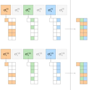
Structure lemmas. Our 1SK-MIFE construction uses index sets to enforce constraints on the adversary’s evaluation (as depicted in Figure 3). The purpose of these constraints is to prevent the adversary from constructing zero-test queries that are inconsistent—i.e., use encodings that “mix and match” elements of different ciphertexts. To show that our design indeed prevents these undesired queries, we first state and prove a few simple definitions and “structure lemmas”, showing that all valid query polynomials have a certain form.

6

Figure 3: The matrices of two1SK-MIFE ciphertexts, ct = (ct(1)₁ ,ct(1)₂ ,ct(1)₃ ) and ct0 = (ct10(1),ct20(1),ct30(1))(both encrypted to slot1), with the index set of each matrix depicted

Definition 5.7(Query-Consistent Polynomials). For an execution trace of the experimentExpt1_P,Q,bSK-MIFE(A)

in the generic multilinear map model, consider any input-consistent sequenceτ = (t1, . . . , tm)of query times

(Definition 4.3). By definition of the encryption procedure, the corresponding ciphertexts for those query times are encoded elements that refer to formal polynomials (Remark 5.6) of the formctti,h=αti,hMˆti,h,

whereαti,his a scalar andMˆti,his aw×wmatrix. We now define the formal polynomial

ατ =

Y

i∈[m], h∈[d]

αti,h

(intuitively, theαcoefficient that would be present, for a given query sequenceτ, in an honest evaluation of the program), as well as the tuple of formal polynomials

ˆ

M|_τ =Mˆ_{tinp(1),inp.h(1)}, . . . ,Mˆ_{tinp(`),inp.h(`)}

(intuitively, the matrices whose entries would be involved in an honest evaluation of the program). Finally, we say that a formal polynomial zτ,bis consistentwith the query sequenceτ if it can be expressed as a

polynomial in the entries of the correct vectors and matrices (ˆs,Mˆ|τ, andˆt), scaled by the correct blinding

coefficient,ατ. More precisely,zτ is consistent withτ if it is identically equal to a formal polynomial of the

form

zτ =ατ·pτ(ˆs, Mˆ|τ, ˆt)

for some polynomialpτ of degreepoly(λ).

Lemma 5.8 (Decomposition of Zero-Test Queries). Fix any efficient adversary A. In the experiment

Expt1_P,Q,bSK-MIFE(A), with all but negligible probability, everyMM.ZeroTestquery made byAthat is valid (i.e., whose handle is at the top-level universeU), refers to a polynomial (Remark 5.6) formally equal to a sum of (potentially exponentially many) query-consistent polynomials of the form

z=X

τ

ατ ·pτ(ˆs, Mˆ |τ, ˆt),

and each polynomialpτ is allowable (Definition 2.6) and consistent with a query sequenceτ (Definition 5.7).

Proof. Consider any valid formal polynomialzsubmitted toMM.ZeroTest. First, we expand the polynomial zinto a sum of monomials (for purposes of analysis, not by the scheme), and collect like terms with respect to theαvariables. Each term in the resulting expression must be encoded at the top-level universeU, since some valid zero-testing handle refers to their sum. This means, in particular, that the index set of each term must contain a partition of everyUi.

The only variables available to the adversary whose index sets contain elements ofUiare the ciphertexts ctt,h generated during time stepst∈ T(i), whereT(i)is the set of all times at which the adversary made

chosen-plaintext queries for input sloti. For these time steps, we will assume that the partitions selected by the challenger:

Pt= (St,(i1), . . . , S (i)

t,d) :t∈ T

(i)

are distinct, since each is drawn independently uniform from a family of size2λ, regardless of the adversary’s queries, and thus by the birthday bound a collision occurs with negligible probability.

This implies that the index setsS_t,h(i)are distinct elements of the exclusive partition familyFit, and thus