ABSTRACT
HAGLUND, NICOLE LYNNE. Quantitative Precipitation Forecast Sensitivity to
Microphysics Parameterization and Sea Surface Temperature Source over North Carolina during Two Cold Season Events. (Under the direction of Gary M. Lackmann.)
In the southeastern United States, some of the most dramatic model quantitative precipitation forecast (QPF) failures in recent years have been associated with winter
precipitation events. For example, the Eta model predicted nearly three inches of total liquid equivalent precipitation over most of central and eastern North Carolina for 2-3 December 2000, while less than 0.10 in. (2.54 mm) of liquid equivalent precipitation actually fell over the majority of central North Carolina. While the over-prediction of precipitation for the 21-22 January 2003 event was not as significant, the predicted precipitation nevertheless might have led to a higher impact case, if it had verified. Despite a forecasted liquid cloud with a cloud top temperature warmer than -15°C, the Eta model produced excessive QPF for both cold season events.
The purposes of this study are (i) to determine whether sea surface temperature data source (1° by 1° weekly Reynolds SST vs. 1.27-km CoastWatch daily SST) could have significantly impacted the 2-3 December 2000 QPF; (ii) to test sensitivities associated with the Ferrier microphysics scheme by studying the effects of various ice nucleation and total glaciation temperatures on QPF; and (iii) to investigate sensitivity of QPF to sea surface temperature data and to choice of microphysics scheme to determine which change yields a more significant contribution to QPF differences.
testing the QPF differences due to choice of microphysics parameterization scheme and to choice of sea surface temperature (SST) data source for the 2-3 December 2000 case, while only the sensitivity of QPF to choice of microphysics parameterization scheme was tested for the 21-22 January 2003 case. It was hypothesized that by cooling the ice nucleation and total glaciation temperatures, better QPF (less precipitation with a cooler ice nucleation
temperature, more precipitation with a cooler total glaciation temperature) would result in both cases. Since the cloud top temperature in the 21-22 January 2003 case was below the original total glaciation temperature (-10°C), cooling the total glaciation temperature was not expected to change the QPF. Additionally, for the 2-3 December 2000 case, it was
hypothesized that changes in SST data source would have a greater impact than the choice of microphysics parameterization scheme on QPF.
Major findings in this study include: (i) Surface low tracks and total precipitation patterns were not significantly different between the runs using Reynolds SST and
CoastWatch SST data; (ii) By cooling the ice nucleation temperature in both case studies, better (closer to analyzed) QPF resulted in the 21-22 January 2003 case. With a cooler total glaciation or ice nucleation temperature in the 2-3 December 2000 case, no clear QPF difference pattern emerged; (iii) While a qualitative analysis of total liquid-equivalent precipitation differences between SST data source and microphysics parameterization scheme runs indicated that SST data source had a greater impact on QPF than choice of microphysics scheme, area-averaged total liquid-equivalent precipitation in three regions showed that choice of SST data source led to QPF biases on the same order of magnitude as the QPF biases due to choice of microphysics scheme; and (iv) Since there are more
subsequent version) than there are between the two versions using any microphysics scheme, choice of microphysics scheme has less of an impact on QPF than convective
BIOGRAPHY
Nicole Lynne Haglund was born in Kansas City, Missouri and grew up in Blue Springs, Missouri. Severe storms terrified her until a local broadcast meteorologist came to her elementary school. The broadcast meteorologist explained that he had been afraid of storms and that when he learned more about them, he was no longer afraid. Following his advice, she learned about storms, lost her fear, and became obsessed with weather. The first tornado she recalls seeing was down the street from her house during her one year in
Livermore, California, during the 1997-1998 El Nino season.
In the fall of 2000, Nicole began her undergraduate study at the University of Oklahoma with plans of becoming a broadcast meteorologist like her childhood mentor. However, by the time Nicole completed her Bachelor’s degree, she had decided that research and forecasting were more interesting. As an undergraduate, Nicole was an active participant in the University of Oklahoma Student Chapter of the American Meteorological Society, an administrator for the student-run forecasting lab (the Oklahoma Weather Lab), and a trained storm spotter. During the summer and winter breaks, starting May 2002 and ending August 2004, Nicole was a SCEP intern at the Aviation Weather Center in Kansas City. While she was an intern, she was trained on each of the desks, completed turbulence research, and repaired/created NAWIPS products for the forecasters.
After graduating with a major in meteorology and a minor concentration in
2005, Nicole began her Master’s work under the CSTAR project, collaborating with the Environmental Modeling Center (EMC) to improve winter storm forecasting. Upon
ACKNOWLEDGMENTS
This research was supported by the NOAA Collaborative Science, Technology, and Applied Research (CSTAR) program (Grant # NA03NWS4680007) awarded to North Carolina State University, as well as the National Science Foundation (NSF) Grant #ATM0342691.
The National Center for Atmospheric Research (NCAR) is acknowledged for the availability of the Weather Research and Forecasting (WRF) model. Other data sources that have been invaluable to this study include: the Comprehensive Large Array-data Stewardship System (CLASS) that provides archived high-resolution sea surface temperature data, the National Centers for Environmental Prediction (NCEP) meteorological data, the North Carolina State Climate Office cooperative observers network liquid-equivalent precipitation data, and the NOAA National Operational Model Archive and Distribution System
(NOMADS) that provides the North American Regional Reanalysis (NARR) and Reynolds SST 1 degree grids. Thank you to Ryan Torn of University of Washington for the original WRF to GEMPAK converter.
Lackmann, for his encouragement when I needed it most, his unfailing optimism, and his patience with my frequent questions.
Second, I would like to thank my labmates (Kevin Hill, Tom Green, Megan Gentry, Blair Holloway, Kelly Mahoney, and Dr. Michael Brennan), who made my graduate school experience entertaining. Not only did we work together in the Forecasting Lab, sharing tips and tricks, but we also spent some of our free time together. Two labmates in particular deserve special thanks: Kelly Mahoney and Dr. Michael Brennan. It would have been impossible to conduct my research without their help in WRF, Fortran, and general computing. Without the immense help of Matt Borkowski and his high-resolution sea surface temperature guide, I would not have been able to complete my sea surface
temperature sensitivity tests. I would also like to share my appreciation of the support and friendship of the RIII and Jordan Hall grad students, especially Jerilyn Billings, Chad Ringley, Emily Lunde, and Patrick Pyle.
TABLE OF CONTENTS
LIST OF TABLES……….. xi
LIST OF FIGURES………..……….. xii
1. INTRODUCTION……….… 1
1.1 Motivation………...…... 1
1.2 Background Research……….…… 3
1.2.1 Microphysics and Microphysics Parameterization………... 4
1.2.2 Sea Surface Temperature Data……….… 8
1.3 Hypotheses……….… 11
1.3.1 Microphysics……… 11
1.3.2 Sea Surface Temperature Data……….… 14
2. DATA AND METHODOLOGY………..… 18
2.1 Weather Research and Forecast (WRF) Model……….… 18
2.1.1 Ferrier Microphysics Scheme……….. 20
2.1.2 Kessler Microphysics Scheme……….. 20
2.1.3 Thompson Microphysics Scheme……….… 20
2.1.4 WSM6 Microphysics Scheme……….. 21
2.2 Data……….. 21
2.2.1 NARR Data……….. 21
2.2.2 Sea Surface Temperature Data……….… 23
2.2.2.1 1° by 1° (Low-Resolution)……… 23
2.2.2.2 1.27-km (High-Resolution)………... 23
2.4 Simulated Radar Reflectivity………... 25
2.5 CFAD Plots……….. 25
2.6 Observational Analysis Used to Choose Cases……….... 26
2.7 WRF Sensitivity Tests……….…. 28
2.7.1 Microphysics Ice Nucleation/Total Glaciation Temperature Sensitivity………..……... 28
2.7.2 Sea Surface Temperature Data Resolution Sensitivity………. 29
3. CASE STUDIES……… 40
3.1 Case Study 1: 2-3 December 2000………... 40
3.1.1 Case Overview………. 40
3.1.2 Microphysics Sensitivity Tests (26.9-km Runs)……….…………. 43
3.1.2.1 Motivation……….... 43
3.1.2.2 Hypothesis……….... 43
3.1.2.3 Eta Forecast……….. 44
3.1.2.4 WRF Model Simulations……….. 44
3.1.2.5 Results……….. 45
3.1.2.5.1 Model Forecast Soundings………. 45
3.1.2.5.2 Model CFAD Comparisons……… 47
3.1.2.5.3 Four-panel Plots………. 53
3.1.2.5.3.1 SLP Comparison……….... 54
3.1.2.5.3.2 Total Precipitation Comparison……….. 55
3.1.2.5.3.3 Total Precipitation Difference Plots…... 56
3.1.3 Correction of the “Ferrier Anomaly” and Sensitivity to Convective
Parameterization Scheme……….. 92
3.1.3.1 The “Ferrier Anomaly,” Model Changes, and Expected Results……….. 92
3.1.3.2 Microphysics Parameterization Comparison Between V2.1.2 and New WRF Runs………. 94
3.1.3.2.1 Shortwave Radiation and 2-m Temperature Plots……… 94
3.1.3.2.2 Simulated Soundings……….. 96
3.1.3.2.3 Four-Panel Plots……….. 97
3.1.3.2.3.1 SLP Comparison..……… 98
3.1.3.2.3.2 Total Precipitation Comparison ……….. 99
3.1.3.2.4 Total Precipitation Area Average Findings……. 102
3.1.3.3 Convective Parameterization Scheme Sensitivity Comparison Between V2.1.2 and New WRF Runs…….………. 104
3.1.3.3.1 6-hr Convective Precipitation, Potential Vorticity, and SLP Comparison………. 104
3.1.3.4 Summary of New Runs……… 105
3.1.4 Sea Surface Temperature Data Sensitivity Tests (12-km Runs)….. 128
3.1.4.1 Motivation……… 128
3.1.4.2 Hypothesis……… 128
3.1.4.3 WRF Model Simulations……….. 128
3.1.4.4.1 Low Resolution SST Plots……….. 129
3.1.4.4.2 High Resolution SST Plots……….… 130
3.1.4.4.3 Difference Plots……….. 132
3.1.4.4.4 Total Precipitation Area Average Findings …... 136
3.1.5 Case Summary……….… 138
3.2 Case Study 2: 21-22 January 2003……… 161
3.2.1 Case Overview……….. 161
3.2.2 Microphysics Sensitivity Tests (26.9-km Runs)……….. 163
3.2.2.1 Motivation……… 163
3.2.2.2 Hypothesis……… 163
3.2.2.3 Eta Forecast……….. 164
3.2.2.4 WRF Model Simulations……….. 164
3.2.2.5 Results……….. 165
3.2.2.5.1 Model Forecast Soundings………. 165
3.2.2.5.2 Four-panel Plots……….. 167
3.2.2.5.2.1 SLP Comparison……….… 167
3.2.2.5.2.2 Total Precipitation Comparison………. 168
3.2.2.5.2.3 Total Precipitation Difference Plots…... 168
3.2.2.5.3 Total Precipitation Area Average Findings …... 169
3.2.3 Case Summary……….. 170
4. DISCUSSION AND CONCLUSIONS……….… 202
4.1 Discussion of Main Results/Conclusions……… 202
4.1.2 Case Studies……….. 204
4.1.2.1 Case 1: 2-3 December 2000………. 204
4.1.2.2 Case 2: 21-22 January 2003………. 208
4.1.3 Final Thoughts……….. 209
4.2 Future Work………. 212
LIST OF TABLES
Table 2.1 Number of Grid Points Used in Area Averaging……….…. 33 Table 2.2 Number of Grid Points Per Level in Model CFADs………. 35 Table 2.3 List of WRF Simulations……….. 39 Table 3.1 ETA Fous data and total QPF in inches for Raleigh-Durham (RDU),
based on Badgett (2006)………... 63 Table 3.2 Area Average Total Liquid-Equivalent Precipitation (in) During 2-3
December 2000 Event — 26.9-km WRF Microphysics Sensitivity Test
Runs……….. 91 Table 3.3 Area Average Total Liquid-Equivalent Precipitation (in) During 2-4
December 2000 Event—26.9-km New WRF Microphysics Sensitivity
Test Runs………... 125
Table 3.4 Area Average Total Liquid-Equivalent Precipitation (in) During 2-3
December 2000 Event—12-km WRF SST Sensitivity Test Runs………… 160 Table 3.5 Area Average Total Liquid-Equivalent Precipitation (in) Biases During
2-3 December 2000 Event—12-km WRF SST Sensitivity Test Runs……. 161 Table 3.6 Area Forecast Discussion for Raleigh and north-central North Carolina at
1725 UTC 20 January 2003……….. 185 Table 3.7 Area Average Total Liquid-Equivalent Precipitation (in) During 21-22
January 2003 Event — 26.9-km WRF Microphysics Sensitivity Test
LIST OF FIGURES
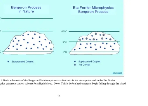
Figure 1.1 Basic schematic of the Bergeron-Findeisen process as it occurs in the atmosphere and in the Eta Ferrier microphysics parameterization scheme for a liquid cloud. Note: This is before hydrometeors begin falling through
the cloud..……….…………. 16
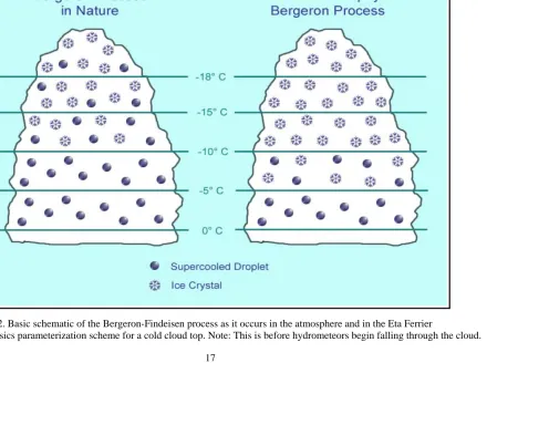
Figure 1.2 Basic schematic of the Bergeron-Findeisen process as it occurs in the atmosphere and in the Eta Ferrier microphysics parameterization scheme for a cold cloud top. Note: This is before hydrometeors begin falling
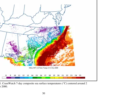
through the cloud ……….… 17 Figure 2.1 CoastWatch 7-day composite sea surface temperatures (°C) centered
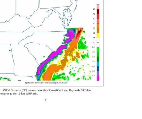
around 2 December 2000……….…. 30 Figure 2.2 SST differences (°C) between modified CoastWatch and Reynolds SST
data after interpolation to the 12-km WRF grid………... 31 Figure 2.3 Areas used in total precipitation averages centered around (a) Greensboro,
NC (GSO), (b) southeast of Pitt Greenville, NC (SE PGV), and (c) north of Darlington, SC (N UDG)……….. 32 Figure 2.4 Hydrometeor mixing ratio plots for Fer0510, including (a) cloud water,
(b) snow, (c) rain, and (d) graupel……… 34 Figure 2.5 WRF run plot for 2-3 December 2000 case using the BMJ convective
parameterization scheme and WSM6 microphysics parameterization scheme. (a) Total liquid-equivalent precipitation (mm) through 1200 UTC 4 December 2000 (F60), (b) 500-hPa heights (dam) and absolute vorticity (x10-5 s-1) at F42, (c) mean sea level pressure (hPa) and 2-m temperatures (°C) at F42, and (d) total convective precipitation (mm) at F60………….. 36 Figure 2.6 WRF run plot for 2-3 December 2000 case using the KF convective
parameterization scheme and WSM6 microphysics parameterization scheme. (a) Total liquid-equivalent precipitation (mm) through 1200 UTC 4 December 2000 (F60), (b) 500-hPa heights (dam) and absolute vorticity (x10-5 s-1) at F42, (c) mean sea level pressure (hPa) and 2-m temperatures (°C) at F42, and (d) total convective precipitation (mm) at F60………….. 37 Figure 2.7 WRF model domain with 26.9-km grid-spacing used in microphysics
parameterization scheme sensitivity tests………. 38 Figure 2.8 WRF model domain with 12-km grid-spacing used in sea surface
Figure 3.1 Precipitation accumulation map from Badgett et al. (2006) for the 2-3
December 2000 event………... 60 Figure 3.2 Total liquid-equivalent precipitation (inches) for the 2-3 December 2000
event forecasted by the 0000 UTC 2 December 2000 Eta211 run……… 61 Figure 3.3 1200 UTC 2 December Eta211 forecast sounding for Raleigh-Durham
(RDU), valid at 1800 UTC 3 December (F030). Dashed green lines indicate the dewpoint profile (°C), while solid red lines indicate the
temperature profile (°C). Wind barbs are in knots.………... 62 Figure 3.4 WRF (a)Fer0510, (b)Fer0530, (c)Fer1030, (d)Kessl, (e)Thomp, and
(f)WSM6 simulated soundings for RDU, valid at 1800 UTC 3 December (F042). Dashed green lines indicate the dewpoint profile (°C), while solid red lines indicate the temperature profile (°C). Wind barbs are in knots… 64 Figure 3.5 CFAD areas centered over (a) Morehead City, NC (MHX) and (b) Raleigh,
NC (RAX). Straight lines indicate where cross-sections were taken. Orange indicates the Lumberton, NC (LBT) to 34.61 N 74.48 W section, violet indicates the Suffolk, VA (SFQ) to 32.91 N 76.54 W cross-section, blue indicates the Statesville, NC (SVH) to Manteo, NC (MQI) cross-section, and green indicates the Farmville, VA (FVX) to North
Myrtle, SC (CRE) cross-section……….. 65 Figure 3.6 Statesville, NC (SVH) to Manteo, NC (MQI) cross-sections of
(a) Thompson cloud ice (blue) and cloud water (green) in 10-2 g/kg, (b) WSM6 cloud ice and cloud water (10-2 g/kg), (c) Thompson
hydrometeor mixing ratios (blue=snow, magenta=graupel, green=rain) in g/kg, and (d) WSM6 hydrometeor mixing ratios (g/kg). The red dashed line indicates the freezing level………... 66 Figure 3.7 Statesville, NC (SVH) to Manteo, NC (MQI) cross-section of omega
(blue=descent, red=ascent) for (a) Thompson and (b) WSM6……… 67 Figure 3.8 Vertical motion (red dashed line=descent, blue solid line=ascent) for the
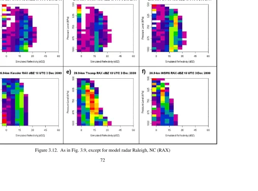
SVH-MQI Thompson cross-section……… 68 Figure 3.9 Simulated reflectivity (dBZ) CFADs produced by (a) Fer0510, (b) Fer0530,
(c) Fer1030, (d) Kessler, (e) Thompson, and (f) WSM6 WRF runs at the Morehead City, NC (MHX) model radar site. Red indicates the highest concentration of gridpoints having a particular reflectivity range (dBZ) at a particular pressure level (hPa), while white indicates the lowest
Figure 3.10 Contoured Frequency by Altitude Diagrams (CFADs) of rain mixing ratio (QRAI) produced by the (a) Kessler, (b) Thompson, and (c) WSM6 WRF runs at the MHX model radar. Red indicates the highest concentration of gridpoints having a particular rain mixing ratio range (g/kg) at a particular pressure level (hPa), while white indicates the lowest concentration of gridpoints. The ordinate labels are shifted up and the abscissa labels are shifted to the right, both by 1 unit. The hydrometeor mixing ratio bin size
is 0.01 g/kg.……….……….. 70
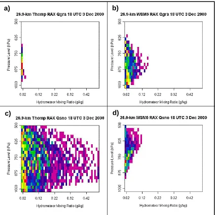
Figure 3.11 CFADs of graupel mixing ratio (QGRA) produced by the (a) Thompson and (b) WSM6 WRF runs and CFADs of snow mixing ratio (QSNO) produced by the (c) Thompson and (d) WSM6 runs. All CFADs are calculated at the model radar site MHX. Red indicates the highest concentration of gridpoints having a particular rain mixing ratio range (g/kg) at a particular pressure level (hPa), while white indicates the lowest concentration of gridpoints. The ordinate labels are shifted up and the abscissa labels are shifted to the right, both by 1 unit. The hydrometeor mixing ratio bin size is 0.01 g/kg……….. 71
Figure 3.12 As in Fig. 3.9, except for model radar Raleigh, NC (RAX)………. 72
Figure 3.13 As in Fig. 3.10, except for model radar RAX………. 73
Figure 3.14 As in Fig. 3.11, except for model radar RAX………. 74
Figure 3.15 0000 UTC 2 December 2000 Eta211 run 4-panel plot showing: (a) Total liquid-equivalent precipitation (inches) through 1200 UTC 4 December 2000 (F60), (b) 500-hPa heights (dam) and absolute vorticity (x10-5 s-1) at 1800 UTC 3 December 2000 (F42), (c) mean sea level pressure (hPa) and 2-m temperatures (°C) at F42, and (d) 250-hPa winds (m/s) at F42………. 75
Figure 3.16 NARR 4-panel plot showing: (a) Total liquid-equivalent precipitation (inches) through 1200 UTC 4 December 2000, (b) 500-hPa heights (dam) and absolute vorticity (x10-5 s-1) at 1800 UTC 3 December 2000, (c) mean sea level pressure (hPa) and 2-m temperatures (°C) at 1800 UTC 3 December 2000, and (d) 250-hPa winds (m/s) at 1800 UTC 3 December 2000………... 76
Figure 3.18 As in Fig. 3.17, except for Fer0530 run……… 78
Figure 3.19 As in Fig. 3.17, except for Fer1030 run……… 79
Figure 3.20 As in Fig. 3.17, except for Kessler run………. 80
Figure 3.21 As in Fig. 3.17, except for Thompson run……… 81
Figure 3.22 As in Fig. 3.17, except for WSM6 run………. 82
Figure 3.23 Sea level pressure and 2-m temperature analysis at 1800 UTC 3 December 2000. Isotherms (°C) are shown as dashed red lines and isobars (hPa) are represented by solid black lines……… 83
Figure 3.24 Sea level pressure and 2-m temperature analysis for 1800 UTC 3 December 2000, with surface and ship/buoy observations overlaid. Solid lines denote sea level pressure (hPa) and dashed lines represent 2-m temperatures (°C)……… 84
Figure 3.25 Total liquid-equivalent precipitation (inches) for 2-4 December 2000 (ending at 1200 UTC 4 December 2000, F60) simulated by: (a) Fer0510, (b) Fer0530, (c) Fer1030, (d) Kessler, (e) Thompson, and (f) WSM6 26.9- km WRF runs initialized at 0000 UTC 2 December 2000………... 85
Figure 3.26 26.9-km WRF total liquid-equivalent precipitation (inches) difference fields for (a) Fer0510 minus Fer0530 and (b) Fer0530 minus Fer1030 runs for the 2-3 December 2000 event. Warm values indicate more total precipitation in the first run than in the second run, while cool colors show less total precipitation in the first run than in the second run………... 86
Figure 3.27 As in Fig. 3.26, except for (a) Kessler minus Fer0510 and (b) Kessler minus Fer1030……….. 87
Figure 3.28 As in Fig. 3.26, except for (a) Kessler minus Fer0530 and (b) Thompson minus Fer0530……….. 88
Figure 3.29 As in Fig. 3.26, except for (a) WSM6 minus Fer0510 and (b) WSM6 minus Fer1030……….. 89
Figure 3.31 6-hr convective precipitation (inches) ending at 1800 UTC 3 December 2000 (F42) and sea level pressure (contoured every 2 hPa) at F42 simulated by (a) the new WRF Fer0510 run and (b) the V2.1.2
Fer0510 run………. 107
Figure 3.32 At 1800 UTC 3 December 2000: (a) WRF V2.1.2 Fer0530 2-m temperatures (°C), (b) new WRF Fer0530 2-m temperatures (°C), (c) WRF V2.1.2 Fer0530 incoming shortwave radiation (Wm-2), and (d) new WRF Fer0530 incoming shortwave radiation (Wm-2)……… 108
Figure 3.33 Incoming shortwave radiation difference (Wm-2) between WRF V2.1.2 Fer0530 and new WRF Fer0530 at 1800 UTC 3 December 2000. Cool colors indicate areas where more shortwave radiation is reaching the surface in new WRF Fer0530 than in WRF V2.1.2 Fer0530………... 109
Figure 3.34 New WRF (a)Fer0510, (b)Fer1030, (c)Fer0530, (d)Kessl, (e)Thomp, and (f)WSM6 simulated soundings for RDU, valid at 1800 UTC 3 December (F042). Dashed green lines indicate the dewpoint profile (°C), while solid red lines indicate the temperature profile (°C). Wind barbs are in knots……… 110
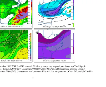
Figure 3.35 0000 UTC 2 December 2000 new WRF Fer0510 run with 26.9-km grid-spacing. 4-panel plot shows: (a) Total liquid-equivalent precipitation (inches) through 1200 UTC 4 December 2000 (F60), (b) 500-hPa heights (dam) and absolute vorticity (x10-5 s-1) at 1800 UTC 3 December 2000 (F42), (c) mean sea level pressure (hPa) and 2-m temperatures (°C) at F42, and (d) 250-hPa winds (m/s) at F42………. 111
Figure 3.36 As in Fig. 3.35, except for new Fer0530 run……… 112
Figure 3.37 As in Fig. 3.35, except for new Fer1030 run……… 113
Figure 3.38 As in Fig. 3.35, except for new Kessler run………. 114
Figure 3.39 As in Fig. 3.35, except for new Thompson run……… 115
Figure 3.40 As in Fig. 3.35, except for new WSM6 run……….. 116
Figure 3.42 Total liquid-equivalent precipitation (inches) for 2-4 December 2000 (ending at 1200 UTC 4 December 2000, F60) simulated by: (a) Fer0510, (b) Fer0530, (c) Fer1030, (d) Kessler, (e) Thompson, and (f) WSM6 26.9- km new WRF runs initialized at 0000 UTC 2 December 2000………….... 118 Figure 3.43 Total liquid-equivalent precipitation difference (inches) between the
V2.1.2 Fer0510 and new WRF Fer0510 runs. Cool colors indicate more total liquid-equivalent precipitation in the new WRF Fer0510 run than in the V2.1.2 Fer0510 run……… 119 Figure 3.44 26.9-km new WRF total liquid-equivalent precipitation (inches) difference
fields for (a) Fer0510 minus Fer0530 and (b) Fer0530 minus Fer1030 runs for the 2-3 December 2000 event. Warm values indicate more total
precipitation in the first run than in the second run, while cool colors show less total precipitation in the first run than in the second run………... 120 Figure 3.45 Total liquid-equivalent precipitation (inches) 3-hr differences between the
new WRF Fer0510 and Fer0530 runs (cooler total glaciation temperature) ending at: (a) F33 (0900 UTC 3 Dec), (b) F36 (1200 UTC 3 Dec), (c) F39 (1500 UTC 3 Dec), and (d) F42 (1800 UTC 3 Dec). The small triangles near the edge of the ovals in (b) and (c) indicate Site1, while the small
squares indicate Site 2.………. 121
Figure 3.46 As in Fig. 3.45, except for new WRF Fer0530 and Fer1030 runs (cooler ice nucleation temperature)..………. 122 Figure 3.47 At 1200 UTC 3 December (F36), new WRF (a) Fer0510 simulated
sounding at Site 1, (b) Fer0530 simulated sounding at Site 1, (c) Fer1030 simulated sounding at Site 1, (d) Fer0510 simulated sounding at Site 2, (e) Fer0530 simulated sounding at Site 2, and (f) Fer1030 simulated
sounding at Site 2……….. 123 Figure 3.48 As in Fig. 3.47, except at 1500 UTC 3 December 2000 (F39)………. 124 Figure 3.49 V2.1.2 Fer0510 sea level pressure with (a) 6-hr convective precipitation
(inches) and (b) 900-700-hPa PV (PVU, where 1 PVU =
1x10⁻⁶ m2 s-1 K kg-1), valid at 1800 UTC 3 December 2000………. 126 Figure 3.50 As in Fig. 3.49, except for new WRF Fer0510 run………... 127 Figure 3.51 Reynolds SST data (1° by 1°) contoured every degree (Celsius), with ship
Figure 3.52 As in Fig. 3.51, except for modified CoastWatch SST data (2.7-km grid-spacing) with Reynolds SST data used to fill in cloud contamination and other gaps. The discontinuity in SSTs east of Virginia is where the modified CoastWatch SST data ends. The SST data have already been
interpolated to the WRF 12-km grid………. 142
Figure 3.53 0000 UTC 2 December 2000 WRF KesslLo run with 12-km grid-spacing. 4-panel plot shows: (a) Total liquid-equivalent precipitation (inches) through 1200 UTC 4 December 2000 (F60), (b) 500-hPa heights (dam) and absolute vorticity (x10-5 s-1) at 1800 UTC 3 December 2000 (F42), (c) mean sea level pressure (hPa) and 2-m temperatures (°C) at F42, and (d) 250-hPa winds (m/s) at F42……… 143
Figure 3.54 As in Fig. 3.53, except for ThompLo run………. 144
Figure 3.55 As in Fig. 3.53, except for WSM6Lo run………. 145
Figure 3.56 Total liquid-equivalent precipitation (inches) for 2-4 December 2000 (ending at 1200 UTC 4 December 2000, F60) simulated by: (a) KesslLo, (b) ThompLo, and (c) WSM6Lo 12-km WRF runs initialized at 0000 UTC 2 December 2000……….. 146
Figure 3.57 As in Fig. 3.53, except for KesslHi run……… 147
Figure 3.58 As in Fig. 3.53, except for ThompHi run………. 148
Figure 3.59 As in Fig. 3.53, except for WSM6Hi run………. 149
Figure 3.60 As in Fig. 3.56, except for (a) KesslHi, (b) ThompHi, and (c) WSM6Hi… 150 Figure 3.61 12-km WRF total liquid-equivalent precipitation (inches) difference fields for (a) KesslLo minus ThompLo and (b) KesslLo minus WSM6Lo runs for the 2-3 December 2000 event. Warm values indicate more total precipitation in the first run than in the second run, while cool colors show less total precipitation in the first run than in the second run………... 151
Figure 3.62 Total liquid-equivalent precipitation (inches) for 2-4 December 2000 (ending at 1200 UTC 4 December 2000, F60) simulated by: (a) KesslLo, (b) ThompLo, (c) WSM6Lo, (d) KesslHi, (e) ThompHi, and (f) WSM6Hi 12-km WRF runs initialized at 0000 UTC 2 December 2000……….. 152
Figure 3.64 12-km WRF total liquid-equivalent precipitation (inches) difference fields for KesslHi minus KesslLo runs for the 2-3 December 2000 event. Warm values indicate more total precipitation in the first run than in the second run, while cool colors show less total precipitation in the first run than in
the second run………... 154
Figure 3.65 As in Fig. 3.64, except for ThompHi minus ThompLo……… 155 Figure 3.66 As in Fig. 3.64, except for WSM6Hi minus WSM6Lo……… 156 Figure 3.67 Eta forecast and WRF simulations surface low track map for the 2-3
December 2000 event. Low centers are plotted every 6 hours from 1200 UTC 2 December to 0000 UTC 4 December. Warm color tracks are from Hi runs, while cool color tracks are from Lo runs……… 157 Figure 3.68 SLP (hPa) difference plot between KesslHi and KesslLo at 1800 UTC 3
December 2000. Solid lines indicate KesslHi SLP pressure, contoured
every 2-hPa……….. 158
Figure 3.69 SST gradient field (°C/100-km) for (a) Reynolds SST and (b) modified CoastWatch SST data. Fill intervals vary since the gradients in the modified CoastWatch SST data have a much higher magnitude (greater than 4 times) than those in the Reynolds SST data. High values along coastlines (at least partly on-shore) are caused by land-sea mask
problems……… 159
Figure 3.70 Total liquid-equivalent precipitation (inches) contoured from rain gauge data for the 21-22 January 2003 event……….. 172 Figure 3.71 (a) Hourly precipitation amounts (inches) contoured from rain gauge data,
Figure 3.77 Radar reflectivity (dBZ) around 1900 UTC 21 January 2003……….. 179 Figure 3.78 Sea level pressure and 2-m temperature analysis with observations
overlaid at 1800 UTC 21 January 2003. Heavy solid lines represent
isobars (hPa) and dashed lines represent isotherms (°C)……….. 180 Figure 3.79 0000 UTC 21 January Eta211 forecast sounding for Greensboro, NC
(GSO), valid at 1800 UTC 21 January (F018). Dashed green lines indicate the dewpoint profile (°C), while solid red lines indicate the
temperature profile (°C). Wind barbs are in knots………... 181 Figure 3.80 Total liquid-equivalent precipitation (inches) for the 21-22 January 2003
event forecasted by the 0000 UTC 21 January 2003 Eta211 run……….… 182 Figure 3.81 Observed soundings at GSO at (a) 1200 UTC 21 January and (b) 0000
UTC 22 January 2003 (from University of Wyoming). Dewpoint and
temperature profiles are in °C and wind barbs are in knots……….. 183 Figure 3.82 0000 UTC 21 January 2003 Eta211 run 4-panel plot showing: (a) Total
liquid-equivalent precipitation (inches) through 1200 UTC 22 January 2003 (F36), (b) 500-hPa heights (dam) and absolute vorticity (x10-5 s-1) at 1800 UTC 21 January 2003 (F18), (c) mean sea level pressure (hPa)
and 2-m temperatures (°C) at F18, and (d) 250-hPa winds (m/s) at F18….. 184 Figure 3.83 As in Fig. 3.78, except at 0000 UTC 22 January 2003………. 186 Figure 3.84 WRF (a)Fer0510, (b)Fer0530, (c)Fer1030, (d)Kessl, (e)WSM6 simulated
soundings and (f) NARR sounding at Greensboro, NC (GSO), valid at 1800 UTC 21 January 2003 (F18). Dashed green lines indicate the dewpoint profile (°C), while solid red lines indicate the temperature
profile (°C). Wind barbs are in knots………... 187 Figure 3.85 As in Fig. 3.84, except for Raleigh-Durham (RDU)………. 188 Figure 3.86 As in Fig. 3.79, except at RDU………. 189 Figure 3.87 0000 UTC 21 January 2003 WRF Fer0510 run with 26.9-km grid-
spacing. 4-panel plot shows: (a) Total liquid-equivalent precipitation (inches) through 1200 UTC 22 January 2003 (F36), (b) 500-hPa heights (dam) and absolute vorticity (x10-5 s-1) at 1800 UTC 21 January 2003 (F18), (c) mean sea level pressure (hPa) and 2-m temperatures (°C) at
Figure 3.89 As in Fig. 3.87, except for Fer1030 run……… 192 Figure 3.90 As in Fig. 3.87, except for Kessler run………. 193 Figure 3.91 As in Fig. 3.87, except for WSM6 run……….. 194 Figure 3.92 NARR 4-panel plot showing: (a) Total liquid-equivalent precipitation
(inches) through 1200 UTC 22 January 2003, (b) 500-hPa heights (dam) and absolute vorticity (x10-5 s-1) at 1800 UTC 21 January 2003, (c) mean sea level pressure (hPa) and 2-m temperatures (°C) at 1800 UTC 21 January 2003, and (d) 250-hPa winds (m/s) at 1800 UTC 21
January 2003………. 195
Figure 3.93 Total liquid-equivalent precipitation (inches) for 21-22 January 2003 (ending at 1200 UTC 22 January 2003, F36) simulated by: (a) Fer0510, (b) Fer0530, (c) Fer1030, (d) Kessler, and (e) WSM6 26.9-km WRF
runs initialized at 0000 UTC 21 January 2003, and (f) NARR.…………... 196 Figure 3.94 26.9-km WRF total liquid-equivalent precipitation (inches) difference
fields for (a) Fer0510 minus Fer0530 and (b) Fer0530 minus Fer1030 runs for the 21-22 January 2003 event. Warm values indicate more total precipitation in the first run than in the second run, while cool colors
show less total precipitation in the first run than in the second run……….. 197 Figure 3.95 26.9-km WRF total liquid-equivalent precipitation (inches) difference
field for Kessler minus Fer0510 for the 21-22 January 2003 event. Warm values indicate more total precipitation in the first run than in the second run, while cool colors show less total precipitation in the
first run than in the second run……….. 198 Figure 3.96 As in Fig. 3.95, except for Kessler minus Fer1030………... 199 Figure 3.97 As in Fig. 3.94, except for (a) WSM6 minus Fer0510 and (b) WSM6
1. INTRODUCTION 1.1 Motivation
Despite advances in technology and knowledge, quantitative precipitation forecasting (QPF) remains a challenge for numerical weather prediction (NWP) models, as well as for forecasters (e.g., Emanuel et al. 1995; Olson et al. 1995; Fritsch et al. 1998; Zhang et al. 2002; Stoelinga et al. 2003; Roebber et al. 2004). In the southeastern United States, some of the most dramatic model QPF failures in recent years have been associated with winter precipitation events. For example, operational models predicted nearly three inches of total liquid-equivalent precipitation over most of central and eastern North Carolina for 2-3
December 2000, while less than 0.10 in. (2.54 mm) of liquid-equivalent precipitation actually fell over the majority of central North Carolina.
In winter events where the amount of snowfall or freezing precipitation is much greater, large metropolitan areas (such as those along the East Coast) are often severely impacted, leading to mass power outages, transportation problems, and other difficulties. Thus, it is imperative to have reliable QPF, so that timely watches and warnings can be issued, giving towns and municipalities adequate time to prepare. However, models and forecasters may sometimes overforecast precipitation, which may lead to decreased public confidence in the future (Maglaras et al. 1995). One of the cases chosen for this study (2-3 December 2000) had QPF that, had it verified, might have rivaled the 24-25 January 2000 snowstorm, a U.S. East Coast snowstorm in which more than 20.3 in (51.5 mm) of snow fell over Raleigh, North Carolina and surrounding areas (Brennan and Lackmann 2005).
However, the amount of precipitation that fell in the 2-3 December 2000 event was much less than was predicted. While the over-prediction of precipitation for the 21-22 January 2003 event was not as significant, the predicted precipitation nevertheless might have led to a higher impact case, if it had verified.
This study focuses on the sensitivity of the WRF model to microphysics
parameterization schemes and sea surface temperature (SST) data in the 2-3 December 2000 and 21-22 January 2003 winter weather events over the Carolinas. The main purposes of this study are to:
(ii) test sensitivities associated with the Ferrier microphysics scheme by studying the effects of various ice nucleation and total glaciation temperatures on QPF; and
(iii) investigate sensitivity of QPF to sea surface temperature data and to choice of microphysics scheme to determine which change yields a more significant contribution to QPF differences.
It was discovered near the end of this study that there was a problem with cloud radiation-microphysics interactions accompanying the Ferrier scheme implementation in the WRF-ARW model (through WRF version 2.1.2), so a corrected version of the model was obtained and new simulations were run to determine whether the original results were still valid. Section 3.1.3 presents the findings.
The current chapter outlines background research and major hypotheses. Chapter 2 describes methodology, tools, and data utilized in this study. The two case studies and sensitivity study model simulations are presented in Chapter 3, while Chapter 4 provides discussion of the main results, conclusions, and future work.
1.2 Background Research
and sea surface temperature data (one aspect of initial conditions). Section 1.2.1 outlines basic understanding of microphysics as it pertains to this study in terms of ice nucleation and total glaciation temperatures, as well as the Bergeron-Findeisen process. Additionally, some studies using microphysics parameterization sensitivity tests are described. The sensitivity of model QPF and other phenomena to the source and resolution of sea surface temperature data in previous studies is discussed in Section 1.2.2.
1.2.1 Microphysics and Microphysics Parameterization
According to Cantrell and Heymsfield (2005), the chemical and physical principles of ice nucleation are inadequately understood. Even though there is some ostensible agreement between measurements and theory, disagreements between the theories persist. Due to this lack of understanding about microphysical processes, difficulties arise when trying to model ice nucleation and other microphysical processes. In order to simulate microphysical
processes in models, bulk microphysical parameterization schemes are utilized. In these parameterization schemes, the explicit prediction of a limited number of cloud and
precipitation hydrometeor types is based on an array of empirically and theoretically derived sources, sinks, and exchange terms between the hydrometeor types. Despite the relative sophistication of the schemes, flaws in bulk microphysical parameterization schemes are especially apparent in higher-resolution simulations (i.e., Manning and Davis 1997; Colle and Mass 2000).
2001: an offshore frontal precipitation study off the Washington coast, and an orographic precipitation study in the Oregon Cascade Mountains. These data have been used to test mesoscale model simulations of the observed storm systems as well as to evaluate bulk microphysical parameterization schemes used in the models with the hopes of improving model QPF (Stoelinga et al. 2003).
There are two major types of ice nucleation--homogeneous and heterogeneous nucleation. Since the clouds in this study do not extend to the -35°C level, only
heterogeneous nucleation is considered, as homogeneous nucleation occurs at temperatures colder than -35°C (Wallace and Hobbs 2006). Types of heterogeneous nucleation include immersion freezing (the particle that initiates freezing is suspended within the supercooled droplet), contact nucleation (a particle suitable for nucleation comes into contact with a supercooled cloud droplet), deposition nucleation (ice forms by deposition in an environment where air is supersaturated with respect to ice), and condensation-freezing (liquid water condenses onto a suitable particle and then freezes). Condensation-freezing is possible only when the atmosphere is supersaturated with respect to water, while deposition nucleation may occur even in water subsaturated conditions (Wallace and Hobbs 2006).
to –15°C levels and would provide an ample supply of water vapor for the growing ice crystals.
During Project Whitetop, Hoffer and Braham (1962) found that in summertime cumuli ice particles developed by the time the cloud tops reached around –10 to –15°C, while a few clouds began developing ice particles by the time the cloud tops reached –6°C. Total glaciation (all ice cloud) typically occurred 4 to 10 min after the first ice particles were formed. According to Wallace and Hobbs (2006), continental clouds with tops around 0 to –8°C generally contain copious supercooled droplets (Mossop et al. 1967; Koenig 1968; Hobbs 1969; Hobbs and Rangno 1985,1998; Rangno and Hobbs 1991,1994,2001; Korolev et al. 2003), while clouds with tops around –12°C generally have a 50 percent chance of
containing ice, and clouds with tops around –13°C generally have a 100 percent probability of containing ice. Furthermore, the majority of ice nuclei typically do not become active until around –8°C. Thus, if single threshold values for ice nucleation and total glaciation temperatures need to be determined for use in a bulk microphysics parameterization,
observational studies suggest an ice nucleation temperature near –8°C and a total glaciation temperature cooler than –20°C.
Tests of three ice nucleation regimes in the Thompson bulk microphysics scheme revealed little sensitivity when simulating deep and cold cloud systems with cloud-top temperatures less than –25°C, but showed greater sensitivity when simulating shallow, liquid1 cloud systems (warmer than –13°C cloud top). The greatest sensitivity was seen at ice nucleation temperatures between 0 and –10°C (Thompson et al. 2004). Consequently, the
1
choice of ice nucleation temperature may play a significant role in QPF and other fields impacted by microphysical processes.
For liquid clouds (with cloud top temperatures between –5 and –13°C), an ice nucleation temperature of –5°C and a total glaciation temperature of –10°C (the settings in Eta/NAM before 20 June 2006; see NAM 2006 for more details about the change), as set in the Eta Ferrier microphysics parameterization scheme, may introduce mixed-phase
precipitation too readily in the model and lead to complete glaciation faster than would be observed in the atmosphere. Furthermore, supercooled liquid is often found below –10°C, so clouds with cloud-top temperatures between –5 and –10°C often contain all supercooled liquid and little or no ice. This could potentially result in spurious QPF in the model because the Bergeron-Findeisen process is active in the model when it would not be naturally
occurring in the atmosphere. Fig. 1.1 shows a basic schematic of the Bergeron-Findeisen process in the atmosphere versus the Bergeron-Findeisen process as it occurs in the Eta Ferrier microphysics scheme for a liquid cloud, while Fig. 1.2 shows the same comparison, but for a relatively cold cloud top. Note that both schematics depict the initial cloud conditions; when hydrometeors begin to fall through these clouds, the patterns of ice and supercooled liquid will change.
1.2.2 Sea Surface Temperature Data
Since sea surface temperature (SST) influences the atmosphere through its effects on latent and sensible heat fluxes, it is an important parameter both for climate research and for simulations of marine atmospheric boundary layer (MABL) phenomena and associated precipitation in NWP models. One region where SST data are especially important is near the Carolina coast, a favored region for coastal frontogenesis and cyclogenesis due in part to large air-sea temperature differences in the vicinity of strong SST gradients associated with the Gulf Stream (Doyle and Warner 1993). Some studies have suggested that differential heat fluxes near the Gulf Stream are important in coastal frontogenesis near the Carolinas (Bosart and Lin 1984; Riordan 1990; Doyle and Warner 1990), while others (Holt and Raman 1992) found that thermodynamic coupling between the ocean surface and the MABL is an important influence on coastal front structure near the Gulf Stream.
Previous studies have found that simulations of the structure and evolution of coastal mesoscale phenomena such as low-level jets (LLJs), coastal fronts, and coastal cyclones are sensitive to the SST distribution (Mizzi and Pielke 1984;Warner et al. 1990; Jacobs et al. 2005). For example, Lapenta and Seaman (1992) found that when the east-west SST gradient of the Gulf Stream was eliminated, a weaker coastal front and cyclone were produced.
In order to have accurate representation of ocean-atmosphere interaction in operational NWP models, accurate SST fields are essential. Chelton and Wentz (2005) examined various global satellite SST observations, including Advanced Very High
satellite (AMSR-E). AVHRR analyses include Reynolds (weekly 1° by 1° grid) and Real-Time Global SST (RTG_SST) (daily 0.5° by 0.5° grid); the latter analysis is used in the Eta model as of the time of this publication. The study found that in most regions, SST gradients in Reynolds analyses were only 15-25% as strong as in the AMSR-E SST fields (56-km grid-spacing) and SST gradients in RTG_SST analyses were 40-55% as strong as in the AMSR-E fields.
NWP models are sensitive to resolution of SST fields used as surface boundary conditions. While comparing a higher-resolution SST analysis (NOAA 14-km) with a smoothed SST field (Navy’s Feet Numerical Oceanography Center 381-km), Warner et al. (1990) found that the smoothed SST field produced similar MABL responses to those produced by the higher-resolution SST analysis. However, relatively large-scale structures were weaker, with relatively small features frequently being absent. For example, low-level relative vorticity, horizontal velocity, and vertical velocity were all considerably less intense in the smoothed SST run, up to five times weaker than in the higher-resolution SST run. The study also discovered that surface strength of the MABL front was decreased by a factor of four and the maximum 12-h precipitation was less than in the higher-resolution SST run by a factor of two. Similarly, Mailhot and Chouinard (1989) simulated two explosive cyclone cases and found that low-level mesoscale structure was affected substantially when SST analysis was changed from 1° to 2.5° grid-spacing.
Gulf Stream, cool shelf waters, and synoptic and mesoscale features were adequately
simulated. However, with lower resolution runs (MEDIUMSST and COARSESST), the SST gradient was significantly weaker than in FINESST, the cooler shelf waters were either poorly or not resolved at all, and synoptic and mesoscale features were not simulated as well as in FINESST. Due to a lack of cooler shelf waters in COARSESST, there is a maximum in air-sea temperature difference and in sensible and latent heat fluxes just to the east of the Carolina coast. These features produced a simulation closer to FINESST than to
MEDIUMSST, with surface-layer divergence, vorticity, and frontogenesis much more intense in FINESST and COARSESST (two to eight times more intense) than in MEDIUMSST. However, while the coastal phenomena in COARSESST appear more accurate than MEDIUMSST, it is actually an artifact of the greater heat flux gradient in COARSESST near the coast. Due to the contribution by differential diabatic heating, the intensity and positions of the coastal front, cyclone, and associated precipitation varied by SST data source. For example, the main precipitation maximum in eastern North Carolina was 80% and 40% less in MEDIUMSST and COARSESST, respectively, than in FINESST. Therefore, it is essential to use high-resolution SST analyses for accurate prediction of coastal cyclones, fronts, and associated precipitation (Doyle and Warner 1993).
After discovering that choice of model physics can produce a tropical storm of nearly any intensity, Davis and Bosart (2002) caution against tuning of model parameters in order to produce a single simulation that is closer to observations. Instead, they advocate
research was directed toward understanding and attempting to explain QPF sensitivity to choice of microphysics parameterization or SST source.
1.3 Hypotheses
Of the following hypotheses, only the first hypothesis (regarding microphysics) is tested in both case studies. The second hypothesis (regarding sea surface temperature data) is tested only in the 2-3 December 2000 case.
1.3.1 Microphysics
Investigating a liquid cloud case (21-22 January 2003) in which the QPF was over-forecasted over northern North Carolina led to a hypothesis that the Ferrier microphysics parameterization scheme is overactive in liquid cloud cases as compared with the real
atmosphere, where a liquid cloud is defined in this study as a cloud with a top temperature of –15°C and warmer. By cooling the ice nucleation and total glaciation temperatures,it is hypothesized that QPF should more closely resemble observed total precipitation for a cold
season event. With a cooler ice nucleation temperature, a shallower layer of active (in terms
of ice processes) cloud would occur--resulting in reduced QPF as compared with the
original Ferrier run, while a cooler total glaciation temperature would provide more
realistic conditions in which the Bergeron-Findeisen process could occur.
cooler total glaciation temperature, a cloud with a top temperature only slightly cooler than -10°C could be only supercooled water, with no significant amount of ice. Thus, the original Ferrier run, which would have a mixed phase cloud from -5 to -10°C and all ice in the cloud colder than -10°C, would produce more QPF than the run with a cooler total glaciation temperature.
Other kinematic and dynamic fields that may be affected by changes in microphysics in nature include: (i) latent heat release, (ii) mesoscale circulations, and (iii) vertical motion. Released latent heat changes the vertical heating gradient in the regions where condensation or deposition are occurring. With latent heat release, static stability is increased, pressure falls (which induces convergence below the level of maximum heating), and a positive potential vorticity anomaly forms, which enhances cyclonic flow (Hoskins et al. 1985; Thorpe 1985; Bretherton 1966). Since deposition occurs in the Bergeron-Findeisen process, latent heat is released in this process, which could enhance the cyclonic flow below the level of maximum heating. With a positive potential vorticity anomaly at lower levels enhancing cyclonic flow along the North and South Carolina coasts, moisture transport may be
enhanced and more moisture is available to the system, which in turn enhances latent heat release in a positive feedback mechanism akin to that documented by Brennan and
Melting extracts latent heat from the environment, which can lead to organized melting-induced circulations in the vicinity of a rain/snow boundary if there is a horizontal variation of melting rate. These thermally direct mesoscale circulations can consist of forced cold outflow below the melting level and a weaker return flow above (Szeto et al. 1988a,b). As shown in the modeling study by Szeto et al. (1988b), the updraft occurs on the “cold” side of the rain/snow boundary, which would enhance precipitation. With a cooler ice nucleation temperature in a liquid cloud case like the 21-22 January 2003 event (cloud top temperature warmer than -10°C), less model precipitation would be present in the melting layer than if the ice nucleation temperature was warmer. In the latter case, snow/ice is generated by the Bergeron-Findeisen process and melts as it falls into the melting layer, while in the former case, no snow/ice is generated by the Bergeron-Findeisen process in the model (mainly warm cloud processes are active). Thus, horizontal variations of melting rate would not likely occur with a cooler ice nucleation temperature, so the mesoscale circulations would also not be generated.
Small mesoscale wind perturbations within the melting layer can be generated by nonuniform cooling by melting due to spatial variations of precipitation (Atlas et al. 1969). With a horizontal variation in snow distribution above the melting layer, horizontal
temperature > -10°C), no snow would be created in the model, so it is likely that the horizontal gradients of buoyancy would also not occur.
1.3.2 Sea Surface Temperature Data
It is hypothesized that the excessive QPF in the 2-3 December 2000 snowstorm was due only in part to low-resolution, relatively low quality SST data source. Furthermore, it is anticipated that differences in QPF due to choice of microphysics scheme will be less significant than differences in QPF due to choice of SST data source.
enhance precipitation patterns over the land, a low tracking along a baroclinic zone closer to the coast also contributes to more precipitation falling further inland. Thus, SST data source is expected to have an effect on precipitation patterns on-shore.
Jankov et al. (2005) found that the greatest sensitivity in the forecast is due to the choice of convective parameterization scheme, while the least sensitivity is due to the choice of microphysics parameterization scheme. Therefore, it is expected that QPF will be more sensitive to the choice of SST data source than to the choice of microphysics
Figure 1.1. Basic schematic of the Bergeron-Findeisen process as it occurs in the atmosphere and in the Eta Ferrier
Figure 1.2. Basic schematic of the Bergeron-Findeisen process as it occurs in the atmosphere and in the Eta Ferrier
2. DATA AND METHODOLOGY
This chapter describes the data used and the methodology followed in this study. The first section details the Weather Research and Forecast (WRF) model, the model
configuration choices that were made, and the four microphysics parameterization schemes used in the study. The second section describes the data used in the study, the third section explains the area averaging used on the data, the fourth section describes simulated radar reflectivity, the fifth section details contoured frequency by altitude diagrams (CFADs) for the WRF model, the sixth section explains how the two case studies were chosen, and finally, the seventh section details the sensitivity studies for both microphysics parameterization schemes and sea surface temperature data.
2.1 Weather Research and Forecast (WRF) Model
WRF is a flexible mesoscale model designed for both research and operational forecasting that was developed by the National Center for Atmospheric Research (NCAR) and National Centers for Environmental Prediction (NCEP), with assistance from the Forecast Systems Laboratory (FSL), the Air Force Weather Agency (AFWA), the Naval Research Laboratory (NRL), the University of Oklahoma, and the Federal Aviation Administration (FAA). For this study, the following options were used:
(i) Microphysics parameterization schemes: Kessler, Ferrier, Thompson, and WSM6 (Kessler 1969; Ferrier et al. 2002; Thompson et al. 2004; Hong et al. 2004)
(iii) RUC land-surface model (Noah land-surface model, used in the operational WRF/NAM, was not working correctly in WRF version 2.1.2)
(iv) Yonsei University (YSU) PBL scheme (Noh et al. 2003) for the 2-3 December 2000 case; Mellor-Yamada-Janjic (MYJ) PBL scheme (Mellor and Yamada 1982) for the 21-22 January 2003 case (YSU was not working correctly over water in WRF version 2.0.3.1)
(v) Time step of 60 seconds
(vi) Other options were not changed from the “out-of-the-box” 2.1.2 WRF-ARW default namelist settings
Version 2.0.3.1 (see MMM 2006) of the WRF-Advanced Research WRF (ARW) core was used initially, however, the Thompson microphysics parameterization scheme was not implemented in this older version of WRF. Therefore, a newer version (2.1.2) of the ARW core was used for the 2-3 December 2000 case (V2.0.3.1 was still used for the 21-22 January 2003 case, as explained in Section 3.2.2.4). For further details on the WRF model, see Michalakes et al. (2001), Skamarock et al. (2005), Dudhia (2004), and Chen and Dudhia (2006).
this study (one very simple scheme--Kessler; one slightly more complex scheme--Ferrier; and two fairly complex schemes--Thompson and WSM6) are briefly described in the next few sections.
2.1.1 Ferrier Microphysics Scheme
The Ferrier microphysics parameterization scheme (Ferrier et al. 2002) is the operational WRF/Nonhydrostatic Mesoscale Model (NMM) microphysics scheme. It is a relatively simple, very efficient scheme with diagnostic mixed-phase processes. However, in order to achieve its current level of computational efficiency, most physical processes are simplified. Ice nucleation and total glaciation temperatures are set explicitly in the code; current values as of this writing are –5 and –30°C, respectively. However, at the time this study was begun, the ice nucleation and total glaciation temperatures were –5 and –10°C, respectively, in the operational Eta model. As mentioned in Section 1.2.1, the ice nucleation and total glaciation temperatures at these values may potentially lead to excess precipitation. 2.1.2 Kessler Microphysics Scheme
The Kessler microphysics parameterization scheme (Kessler 1969) is a simple, warm-rain (no ice) scheme used often in idealized cloud studies. This scheme was compared with each of the ice schemes. If a model run using an ice-containing scheme is very similar to the output produced when using the Kessler scheme, this suggests that ice processes are not actively generating precipitation.
2.1.3 Thompson Microphysics Scheme
(1962) and Cooper (1986). Ice does not form by the Cooper relationship until the air is saturated with respect to water and the ambient temperature is less than –5°C, or until the water vapor mixing ratio exceeds 5% supersaturation with respect to ice. Ice then continues to form by freezing of cloud droplets (T < -5°C) and by rime-splinter ice production (Hallett and Mossop 1974). This scheme was chosen because it is a new, fairly complex scheme. 2.1.4 WSM6 Microphysics Scheme
The WRF Single Moment 6-class (WSM6) “graupel scheme” (Hong et al. 2004; Hong et al. 2006) has ice, snow, and graupel processes similar to those in the Lin et al. (1983) scheme, but with modified accretion rates (Dudhia 2004). Depending whether the air is supersaturated with respect to ice, ice nucleation may begin at temperatures below 0°C and total glaciation occurs at temperatures below –43°C. Furthermore, the scheme assumes that ice nuclei number concentration is a function of temperature and ice crystal number
concentration is a function of ice amount. WSM6 was chosen as another complex microphysics parameterization scheme.
2.2 Data
2.2.1 NARR Data
reasons: (i) runs using Eta2111, the archived forecast and analysis files for 2-3 December 2000, would not start, and (ii) 32-km grid-spacing in NARR vs. 80-km grid-spacing in Eta211 grids (Rogers et al. 1995) allows for higher resolution initial conditions. For more details about NARR, see Mesinger et al. (2006).
Comparisons of WRF forecast runs using Eta211 analyses as initial conditions with Eta211 forecasts would have been preferable to using NARR for the 2-3 December 2000 case. Using Eta211 analyses would have allowed a more direct comparison of the WRF forecasts to those produced by the Eta, especially since the analysis scheme in Eta was several years older than that used in NARR. However, one of the main purposes of studying the 2-3 December 2000 case was to determine whether or not a higher resolution SST dataset made a significant difference in precipitation amount and location--not studying the changes in QPF due to other initial conditions. Therefore, using the NARR dataset for this study should be sufficient.
The NARR storm total precipitation plots were verified by hand using
liquid-equivalent precipitation totals reported by NWS cooperative observers (not shown). The co-op network was chosen as verification for two major reasons: (i) the Automated Surface Observation System (ASOS) tipping bucket gauge can underestimate the amount of liquid-equivalent precipitation in snow events, by as much as 40-60%, depending on whether or not the gauge is shielded (Colle et al. 2000; NWS 2006), and (ii) there is greater spatial
resolution in the co-op system. Even though the co-op dataset is not ideal because
observations are only available once daily, the cooperative observation system was deemed
1
better for verification than the ASOS tipping bucket gauges. NARR storm totals were determined to be quite close to the liquid-equivalent totals from the co-op data and, more importantly, the total precipitation pattern verified. Therefore, NARR total precipitation was considered sufficient as a source for model verification.
2.2.2 Sea Surface Temperature Data 2.2.2.1 1° by 1° (Low-Resolution)
The relatively low-resolution (1° by 1°) weekly Reynolds SST OI v2.0 was
downloaded from http://nomad3.ncep.noaa.gov/pub/sst/weekly. The Reynolds analysis uses in situ measurements, satellite SSTs, and SSTs simulated by sea ice cover. The satellite data are adjusted for biases using the method of Reynolds (1988) and Reynolds and Marsico (1993). V2.0 refers to the re-computing of optimum interpolation (OI) fields in November 2001 for late 1981 onward. For more details, see Reynolds et al. (2002) and Reynolds and Smith (1994). Since the data files were already in grib format, no conversion was necessary for use in WRF.
2.2.2.2 1.27-km (High-Resolution)
contamination holes. After creating the composite and overlay, the grid-spacing of the data is 2.7-km. Following the conversion to GEMPAK and then to WRF intermediate file format, the high-resolution SST dataset was ingested into WRFSI, and WRF simulations were run. Since the SST data (both high- and low-resolution) are interpolated onto the WRF grids (in this study, using 12- and 27-km grid-spacing), very high-resolution features may be degraded or lost. However, there is still a significant difference between high- and low-resolution SST data, even after interpolation to lower-resolution grids (Fig. 2.2).
2.3 Area Averaging of Total QPF for Each Event
In order to quantitatively examine the total QPF, area averages were computed. Using a FORTRAN program based on an area-averaging program originally written by Kelly Mahoney and Dr. Lackmann, storm total precipitation area averages from WRF runs were computed for areas centered around three points: Greensboro, NC (GSO), southeast of Pitt Greenville, NC (PGV), and north of Darlington, SC (UDG). Fig. 2.3 shows the area covered by each circle of radius 100-km and Table 2.1 shows the number of grid points the
precipitation was averaged over for each area. The GSO area was chosen because the Eta model forecasted more than 2 in (greater than 51 mm) of liquid-equivalent precipitation in that region, but little more than a trace of liquid-equivalent precipitation verified. The Eta model forecasted comparatively less precipitation for the SE PGV and N UDG, but more precipitation verified in this two regions than in the GSO area. In fact, the SE PGV region contains the total precipitation maximum that verified for the case. For 2-3 December 2000, area averages of storm total precipitation were created for each microphysics
NARR analysis at the end of the event. The results of the area averaging are shown in each case study.
2.4 Simulated Radar Reflectivity
In order to look at model-generated hydrometeor mixing ratios and reflectivity, WRF output is post-processed using a radar algorithm in the conversion to GEMPAK files. One of the quantities available in the radar algorithm is “dBZ,” model simulated equivalent
reflectivity factor. The simulated reflectivity values depend upon microphysics parameterization scheme details, especially mixing ratios of hydrometeors.
Currently, hydrometeor mixing ratios are written incorrectly in the WRF-ARW Ferrier scheme; every mixing ratio plot is exactly the same. Fig. 2.4 shows an example of hydrometeor mixing ratio field plots using the Ferrier scheme. This is a post-processing problem, and is not an issue for the model itself.
Possibly the most significant limitations of simulated radar reflectivity are the assumptions required when comparing with actual radar reflectivity. Direct comparisons with current radars are compromised by the following: (i) radar resolution degrades with distance, while model resolution remains constant, (ii) ground clutter and anomalous propagation are present in reality, but are not simulated in models, (iii) models do not simulate the bright band seen in radars, etc (Ferrier et al. 2005).
2.5 CFAD Plots
plotted on the diagram with an ordinate of height/pressure and an abscissa of reflectivity (dBZ) or hydrometeor mixing ratio in this study. Some benefits of this statistical method include: (i) preservation of frequency distribution information, (ii) less sensitivity to
interpretation of radar data at a single point in a volume, and (iii) verification of NWP model results (Yuter and Houze 1995). For more details on CFADs, see Yuter and Houze (1995).
In order to create CFAD plots from WRF model output that may later be compared with radar CFADs in future work, a FORTRAN program was designed to create model CFAD ASCII files. From the ASCII files, both model simulated reflectivity (Ferrier et al. 2005, Stoelinga 2005) and hydrometeor mixing ratio CFADs were created and displayed using the statistical program R. The simulated reflectivity (dBZ) CFAD had 31 levels (every 25-hPa), 13 bins (5 dBZ per bin), with a minimum reflectivity value of 0 dBZ . The
hydrometeor mixing ratio CFAD used 31 levels (every 25-hPa), 49 bins (0.01 g/kg per bin), with a minimum mixing ratio of 0.02 g/kg. Other specifications include two model “radars” with a range (radius) of 230-km, one located at 34.78 N, 76.88 W (location of the Morehead City, NC radar) and the other located at 35.67 N, 78.49 W (location of the Raleigh, NC radar). Table 2.2 shows the number of gridpoints at each vertical level for each of the two model “radar” sites used in the 2-3 December 2000 case study.
2.6 Observational Analysis Used to Choose Cases
model. However, a liquid cloud did not verify, so the case was then used to test the QPF sensitivity of a colder cloud top case to cooler ice nucleation and total glaciation
temperatures. Radar data from the Weather Surveillance Radar-1988 Doppler (WSR-88D) sites were then examined to determine the time periods when precipitation was occurring over North Carolina and to observe how radar echoes in each case progressed with their respective forcing (i.e., precipitation associated with an upper low).
2.7 WRF Sensitivity Tests
In all model runs, thirty-one vertical levels were used. The only changes made were choice of microphysics parameterization scheme (or SST data, depending on the case study) and grid-spacing (either 26.9-km or 12-km, depending on the sensitivity test). Section 2.7.1 details the tests of QPF sensitivity to choice of microphysics parameterization scheme for 26.9-km WRF runs, while Section 2.7.2 describes the tests of QPF sensitivity to choice of high- or low-resolution SST data. After each sensitivity test WRF simulation, the output was converted to a form that could be read and displayed by the General Meteorological Package (GEMPAK, desJardins et al. 1991).
2.7.1 Microphysics Ice Nucleation/Total Glaciation Temperature Sensitivity Tests of QPF sensitivity to microphysics parameterization were run for both case studies, using 26.9-km grid-spacing (see Fig. 2.7 for grid area). At the time of this writing, the Ferrier scheme would not run on the computing system in the same way as the others and had to be run on a single compute node (single processor), rather than using multiple
processors. Even though Ferrier is the most computationally efficient MP scheme, with higher-resolution runs such as 12-km, the process on the compute node currently times out and is killed by the system before the WRF run is complete. Since the Ferrier tests could not be completed for 12-km runs (the current operational grid-spacing in WRF-NMM/NAM), the original 26.9-km test runs were used to compare the Kessler, Thompson, and WSM6
schemes with the Ferrier microphysics parameterization scheme.
(i) Ice nucleation temperature = -5°C, Total glaciation temperature = -10°C (Fer0510 run)
(ii) Ice nucleation temperature = -5°C, Total glaciation temperature = -30°C (Fer0530 run)
(iii) Ice nucleation temperature = -10°C, Total glaciation temperature = -30°C (Fer1030 run)
Before each run, the ice nucleation and total glaciation temperatures were changed in the Ferrier MP scheme FORTRAN program in WRF (module_mp_etanew.F), the model was recompiled, and each simulation was run. Fer0510 represents the temperatures set in the operational Eta before the switch to WRF-NMM (NAM), Fer0530 represents the current temperatures set in NAM, and Fer1030 is an experimental run used to test the ice nucleation temperature.
2.7.2 Sea Surface Temperature Data Resolution Sensitivity
12-km runs (see Fig. 2.8 for grid area) were completed for both data resolutions using Kessler, Thompson, or WSM6 microphysics parameterization schemes. Since each
TABLE 2.1. Number of Grid Points Used in Area Averaging.
SE PGV GSO N UDG
Reanalysis (32-km)
NARR 32 33 32
Forecast (80-km)
Eta211 5 6 4
WRF Runs (26.9-km)
All WRF Runs 44 44 44
WRF Runs (12-km)
a) b)
c)
d)
TABLE 2.2. Number of Grid Points Per Level in Model CFADs.
Raleigh, NC Radar Morehead City, NC Radar
12-km WRF Runs 1156 1157
b)
a)
d)
c)