Software and Methods for Analyzing Molecular Genetic Marker Data

(1)

Abstract

LIU, KEJUN. Software and Methods for Analyzing Molecular Genetic Marker Data (under the direction of DR SPENCER V. MUSE)

(2)

(3)

SOFTWARE AND METHODS FOR

ANALYZING MOLECULAR GENETIC

MARKER DATA

by

KEJUN LIU

A dissertation submitted to the Graduate Faculty of North Carolina State University

in partial fulfillment of the requirements for the Degree of

Doctor of Philosophy BIOINFORMATICS

Raleigh 2003 APPROVED BY:

SPENCER V. MUSE

CHAIR OF ADVISORY COMMITTEE

BRUCE S. WEIR

(4)

(5)

Biography

(6)

Acknowledgements

I would like to express my deepest gratitude to Dr. Spencer V. Muse for being my mentor and guide throughout my graduate studies. His insightful instructions will never go unremembered.

I would also like to thank the members of my advisory committee, Dr. Bruce S. Weir, Dr. Edward Buckler and Dr. Montserrat Fuentes, for their helpful advice and encouragement. They have been a wonderful committee and great resources of valuable ideas which I have found incredibly helpful.

I would like to express my appreciation to all of the members in the maize evolutionary genomics project for their advice and stimulating scientific discussions, especially Dr. John Doebley and Dr. Major Goodman who have been an enormous help to me in both maize genetics and maize evolutionary studies. Special thanks to all of the faculty and staff of the Bioinformatics Research Center. I also thank Doug Robinson, Xiang Yu and Jieye Yu for their friendship and helpful comments.

(7)

List of tables

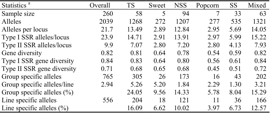
TABLE 2.1:SUMMARY STATISTICS FOR ALL INBREDS AND EACH SUBGROUP... 48

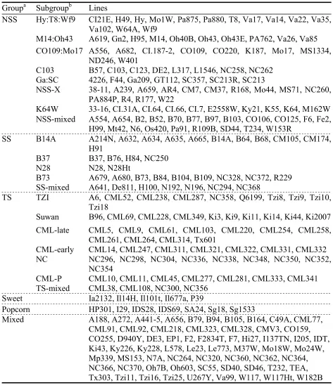
TABLE 2.2: LIST OF THE 260 LINES BY THEIR MODEL-BASED GROUPINGS... 49

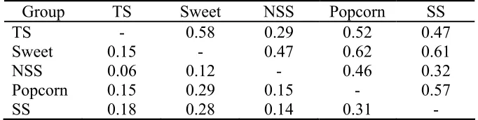
TABLE 2.3: GENETIC DISTANCES BETWEEN MAIZE INBRED GROUPS... 51

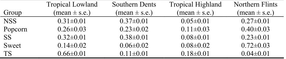
TABLE 2.4: HISTORICAL SOURCES FOR EACH MAIZE INBRED GROUP... 52

TABLE 2.5:LIST OF CORE SETS OF INBRED LINES... 53

TABLE 2.6:PERCENTAGE OF SSR LOCUS PAIRS IN LD AT A p=0.01LEVEL... 54

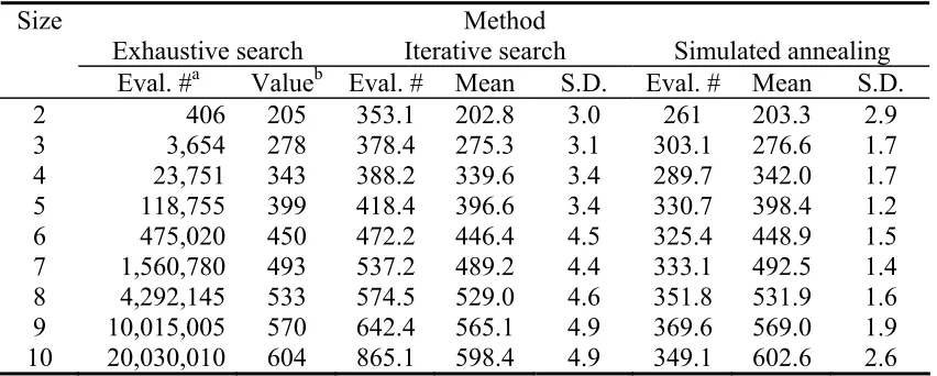
TABLE 3.1: EFFICIENCY OF DIFFERENT OPTIMIZATION ALGORITHMS... 82

TABLE 3.2: EFFICIENCY OF CONSTRAINED OPTIMIZATION... 83

TABLE 3.3: LIST OF 102 MAIZE INBREDS LINES... 84

TABLE 3.4:MAIZE INBREDS CORE SETS IDENTIFIED BY SIMULATED ANNEALING... 85

TABLE 4.1:PERFORMANCE OF RECURSIVE BISECTION ALGORITHM BASED ON |D' |... 118

TABLE 4.2: PERFORMANCE OF RECURSIVE BISECTION ALGORITHM BASED ON r2... 119

TABLE 4.3:ENTROPY VALUES FOR DIFFERENT SETTINGS... 120

(9)

List of figures

FIGURE 2.1: HISTOGRAM OF ALLELE FREQUENCY... 55

FIGURE 2.2: PLOTS OF ALLELE NUMBER OBTAINED AGAINST SAMPLE SIZE... 55

FIGURE 2.3: PLOT OF THE PROPORTION OF SHARED SSR ALLELES DISTANCE BETWEEN INBRED LINES BY THE PEDIGREE DISTANCE BETWEEN INBREDS. ... 55

FIGURE 2.4:FITCH-MARGOLIASH TREE FOR THE 260 INBRED LINES USING THE LOG TRANSFORMED PROPORTION OF SHARED ALLELE DISTANCE... 55

FIGURE 3.1: COMPARISON OF ITERATIVE SEARCH AND SIMULATED ANNEALING. ... 86

FIGURE 3.2: PLOTS OF ALLELE NUMBER OBTAINED AGAINST CORE SET SIZE. ... 86

FIGURE 4.1:RELATIONSHIP BETWEEN AVERAGE NUMBER OF TAGGING SNPS AND NUMBER OF ALL SNPS FOR DIFFERENT RECOMBINATION RATES... 122

FIGURE 5.1: THE OBJECT EXPLORER IN POWERMARKER... 128

FIGURE 5.2: STEP 1 OF DATA WIZARD... 129

FIGURE 5.3:STEP 2 OF DATA WIZARD... 130

FIGURE 5.4: STEP 4 OF DATA WIZARD... 131

FIGURE 5.5: CHOOSE SUBSET DIALOG... 132

FIGURE 5.5: ANALYSIS DIALOG FOR SUMMARY STATISTICS... 133

FIGURE 5.7:TABLE VIEWER IN POWERMARKER... 134

FIGURE 5.8: ANALYSIS DIALOG FOR TWO-LOCUS LINKAGE DISEQUILIBRIUM... 135

FIGURE 5.9: RANGE DIALOG... 136

(10)

Chapter 1

(11)

GENETIC MARKER DATA

The advent of genetic marker technology designed to detect naturally occurring polymorphisms at the DNA level has become an invaluable and revolutionizing tool for both applied and basic diagnostic studies of plant, animal and human genomes as well as for microorganisms. A genetic marker is an identifiable physical location on a chromosome whose inheritance can be monitored. Genetic markers are locus specific and polymorphic in the studied populations. The various established and widely used genetic marker techniques include approaches for detecting restriction fragment length polymorphism (RFLP), randomly amplified polymorphic DNA (RAPD), amplified fragment length polymorphism (AFLP), single nucleotide polymorphism (SNP) and Mini- and Microsatellites (or simple sequence repeats, SSRs).

(12)

region, which can directly influence protein structure or expression levels, giving insights into disease mechanisms. Approximately 90% of human DNA polymorphism, which accounts for a larger fraction of observed differences between individuals, is due to SNPs (Patil et al. 2001).

(13)

MAIZE INBREDS DATA ANALYSIS

(14)

(15)

BLOCK PARTITIONING AND HAPLOTYPE TAGGING

Recent studies suggested the human chromosome appeared to be organized as haplotype blocks. Within these blocks, high linkage disequilibrium (LD) and limited haplotype variation were observed (Patil et al. 2001; Gabriel et al. 2002). The data of haplotype blocks have left several uncertainties concerning the exact block definition and block boundaries. Existing methods for block partitioning are either dependent on haplotype data (Patil et al. 2001) or specific to their applications (Gabriel et al. 2002). In chapter 4, a general algorithm for block partitioning is proposed to maximize the possibility of recombination hotspot identification based on pairwise linkage Disequilibrium (LD). In our method, a block can be defined as a chromosomal region where recombination hotspots do not exist, and the correlation between pairwise LD and physical proximity is not significant. The properties of the algorithm were studied using population simulations.

(16)

POWERMARKER – A SOFTWARE FOR GENETIC DATA ANALYSIS

PowerMarker (http://www.powermarker.net) is an Integrated Analysis Environment (IAE) for genetic marker data. The objective of the software is to provide a comprehensive set of data analysis and data management tools for population genetics researchers. PowerMarker was written in C# to take full advantage of the Microsoft .Net Framework and future platform independence. PowerMarker builds a powerful user interface around both new and traditional statistical methods for population genetic analysis, including summary statistics, population structure, linkage disequilibrium, association tests, coalescence simulation, haplotype estimation, phylogeny, and all the new methods developed in this thesis. PowerMarker is designed to interact seamlessly with Excel, and interacts with TreeView and other population genetic software such as ARLEQUIN and STRUCTURE. We have observed that PowerMarker routines are up to 50 times faster than those in other packages.

(17)

(18)

REFERENCES

Clayton D, Choosing a set of haplotype tagging SNPs from a larger set of diallelic loci. ftp-gene.cimr.cam.ac.uk/software (2001).

Excoffier L, Slatkin M, Maximum-likelihood estimation of molecular haplotype frequencies in a diploid population. Mol Biol Evol 12: 921-927 (1995).

Gabriel SB, Schaffner SF, Nguyen H, Moore JM, Roy J, Blumenstiel B, Higgins J, DeFelice M, Lochner A, Faggart M, Liu-Cordero SN, Rotimi C, Adeyemo A, Cooper R, Ward R, Lander ES, Daly MJ, Altshuler D, The structure of haplotype blocks in the human genome. Science 226: 225-2229 (2002).

Garey MR and Johnson DS, In: Computers and Intractability (Freeman, New York), 222 (1979).

Patil N, Berno AJ, Hinds DA, Barrett WA, Doshi JM, Hacker CR, Kautzer CR, Lee DH, Marjoribanks C, McDonough DP, Nguyen BT, Norris MC, Sheehan JB, Shen N, Stern D, Stokowski RP, Thomas DJ, Trulson MO, Vyas KR, Frazer KA, Fodor SP, Cox DR, Blocks of limited haplotype diversity revealed by high-resolution scanning of human chromosome 21. Science 294: 1719-1723 (2001).

Weir BS and Hill WG. Estimating F-Statistics. Annu. Rev. Genetic. 36, 721-750 (2002) Weir BS and Cockerham CC, Estimating F-statistics for the analysis of population

(19)

Chapter 2 Genetic Structure and Diversity among Maize Inbred Lines as Inferred

from DNA Microsatellites

Kejun Liu1_{, Major Goodman}2_{, Spencer Muse}1_{, J. Stephen Smith}3_{, Ed Buckler}4_{, and} John Doebley5

1

Department of Statistics, North Carolina State University, Raleigh, NC 27695, 2_{Department of Crop Science, North Carolina State University, Raleigh, NC 27695,}

3

Crop Genetics Research and Development, DuPont Agriculture and Nutrition, Pioneer Hi-Bred International, Johnston, IA 50131,

4_{USDA-ARS and Department of Genetics, North Carolina State University, Raleigh, NC} 27695,

(20)

Running Title: Diversity among Maize Inbreds

Key words: maize, Zea, SSR, microsatellite, inbreds

Corresponding Author: John Doebley

445 Henry Mall

Madison, Wisconsin 53705 Phone: 608 265 5803 Fax: 608 262 2976

(21)

ABSTRACT

(22)

INTRODUCTION

Maize (Zea mays L. ssp. mays) inbred lines represent a fundamental resource for studies in maize genetics and breeding. While maize inbreds have been used extensively in hybrid corn productions (Anderson and Brown 1952; Troyer, 2001), they have also been critical for diverse genetic studies including the development of linkage maps (Burr et al.

1988), quantitative trait locus mapping (Edwards et al. 1987; Austin et al. 2001), molecular evolution (Henry and Damerval 1997; Ching et al. 2002), developmental genetics (Poethig 1988; Fowler and Freeling 1996), and physiological genetics (Crosbie

et al. 1978). Most recently, a set of diverse maize inbreds has been employed to perform the first phenotype-genotype association analyses in a plant species (Thornsberry et al.

2002) and estimate linkage disequilibrium in maize (Remington et al. 2002; Tenaillon et al. 2002).

(23)

association analyses requires that population structure among lines be factored into the analysis (Thornsberry et al. 2002).

(24)

MATERIAL AND METHODS Plant Materials

A set of 260 inbred lines representing a sample of the most important public lines from the US, Europe, Canada, South Africa, and Thailand, along with lines from the International Center for the Improvement of Maize and Wheat (CIMMYT) and the International Institute of Tropical Agriculture (IITA) were chosen to represent the diversity available among current and historic lines used in breeding. These include essentially all public lines of importance to temperate breeding and many of the important tropical and subtropical lines. The 260 lines and their pedigrees are listed in Supplemental Table S1. Seed of most lines are still available from their original sources (see http://statgen.ncsu.edu/panzea/), but we have also provided seed samples to both the North Central Regional Plant Introduction Station (NCRPIS) at Ames, IA and to the National Seed Storage Laboratory at Ft. Collins, CO. Most, if not all, lines should be available from the NCRPIS in 2004.

SSR Genotyping

(25)

that are evenly distributed throughout the genome. A list of the SSR loci with their chromosomal locations has been deposited as Supplemental Table S2. Primer sequences are available at the MaizeGDB (http://www.maizegdb.org).

Preanalysis

We began with 264 lines some of which were assayed two to four times for the 100 SSR loci giving a total of 339 assays. Of the 33,900 SSR-genotypes, 4.3% amplified more than one band per inbred line, perhaps because of residual heterozygosity, contamination, or the amplification of similar sequences in two separate genomic regions. In order to minimize the effect of contamination, we dropped seven assays with heterozygosity > 0.20, an unexpectedly high value for maize inbreds. Further, four other assays, which represented the sole assays for four lines, were excluded from the study because their position in a preliminary cluster analysis was strongly discordant with their known pedigrees, suggesting a seed or sample mix-up. We also dropped four loci with mean within-line heterozygosity > 0.10, suggesting that these loci did not faithfully amplify a single locus or that allele-calling was problematic. We dropped two loci with availability (defined as 1 – proportion of missing or null data) < 0.80, suggesting that the locus could not be amplified in the PCR reaction for many lines. The final data set consists of 260 lines and 94 loci.

(26)

consensus genotype was that any allele with frequency > 25% is counted, but if there are three or more alleles that have frequency > 25% then we regard the genotype is missing. The second criterion is that if one assay gave a null phenotype but the other a viable allele, then the inbred was considered homozygous for the visible allele. Since there was a high degree of concordance among assays, inferred consensus genotypes based on these criteria represent only 1.9% of the final data set.

Summary statistics and tests

We used PowerMarker (Liu and Muse 2003) to calculate observed heterozygosity, gene diversity (or expected heterozygosity), number of private alleles, number of group-specific alleles, pairwise F-statistics, and stepwise mutation model (SMM) index. Gene diversity was calculated at each locus as

) 1 2 /( ) 1

(

2_n _p2 _n _f

u

u − −

−

∑

,

where pu is the frequency of the uth allele, n is the sample size, and ƒ is the inbreeding coefficient estimated from genotype frequencies (Weir 1996). SMM index was defined as the maximal proportion of alleles that follow a stepwise mutation pattern (Matsuoka et al. 2002a). Analysis of molecular variation (AMOVA) was performed (Excoffier 1992).

(27)

the relationship of pedigree distance and phylogenetic distance, we used a Mantel test (Mantel 1967) by setting the permutation number to 100,000. Pedigree distances were calculated as 1 - Malécot coefficient of coancestry (Malécot 1948) using pedigree information from a variety of sources (see Supplemental Table S1).

Analysis of genetic structure

Lines were subdivided into genetic clusters using a model-based approach with the software package STRUCTURE (Pritchard et al. 1999). Given a value for the number of subpopulations (clusters), this method assigns lines from the entire sample to clusters in a way that Hardy-Weinberg disequilibrium and linkage disequilibrium (LD) were maximally explained. We excluded seven popcorn lines and five sweet corn lines in this analysis (see Results). At least 6 runs of STRUCTURE were done by setting the number of populations (K) from 1 to 10. For each run, burn-in time and replication number were both set to 500,000. The run with the maximum likelihood was used to assign lines to clusters. Lines with membership probabilities ≥ 0.80 were assigned to clusters; lines with membership probabilities < 0.80 for all groups were assigned to a “mixed” group. The three largest clusters were then further subdivided by the same method.

(28)

of the maize wild relative, teosinte (Zea mays ssp. parviglumis) as the outgroup (Matsuoka et al. 2002b).

Analysis of allelic richness

We wanted to compare the allelic richness in maize inbreds to that in open-pollinated landrace (exotic) accessions to estimate the extent to which our set of 260 inbreds captures the diversity present in maize overall. For comparison, we used a previously published dataset for exotic maize of 193 samples that represent the entire maize germplasm pool (Matsuoka et al. 2002b). To make the comparison of allelic richness of inbreds to exotics, we need to adjust for the inbreeding coefficient since inbreds are mostly homozygous while exotics have a high degree of heterozygosity. We also need to adjust for sample size since our sample has 260 inbreds but only 193 exotics. We used two approaches. First, we compared sets of randomly chosen lines from the inbred and exotic datasets with the same sample sizes. The inbred and exotic genotypes were first broken into alleles to simulate the selfing process. Then, the allele number was counted for randomly drawn samples of size three to 193 in steps of five. Second, we used a parametric simulation to simulate the creation of 260 inbreds from the exotic lines. The inbreeding coefficient (ƒ) for inbreds was estimated to be 0.965. For each locus, we sampled two alleles with replacement to generate a diploid genotype. If the two alleles are the same, then the simulated inbred is made homozygous. If the two alleles are different, then the simulated inbred is made heterozygous with probability 1-ƒ and made

(29)

and other summary statistics were calculated. The summary statistics for these simulated data were compared with the actual inbred data.

Estimating the historical sources for inbreds

In order to estimate the historical sources for each inbred group, we used SSR data for 104 representative accessions from four likely historical germplasm pools: Southern dent, Northern flint, Tropical highland maize, and Tropical lowland maize (Supplemental Table S3; Matsuoka et al. 2002b). We calculated the likelihood of the allelic constitution of an inbred group (e.g. NSS) or specific inbred line given different proportions of ancestry from the four historical germplasm pools. Assuming that the loci are independent, the likelihood is

∏∏ ∑

= = = ∝ 4 1 1 4 1 , ) . ( ) , | ( k a j k n klj k klj lj l lj f p f n p Lik

∑

= = < < 4 1 1 , 1 0 k k k p p

Where a_l is number of alleles at the lth locus, f_klj is the frequency of the jth allele at the

(30)

Defining core sets of inbreds

We developed a new algorithm for building core sets of germplasm by maximizing allelic richness using simulated annealing (Kirkpatrick, Gelatt and Vecchi 1983). Given the complete set of lines (L), the algorithm works by first randomly selecting a subset of lines (l). Each line has a weight (w) based on the number of private alleles in that line. Next, between 1 and the minimum( l, L-l) additional lines are chosen from the remainder of the complete set (unselected lines) based on their weights and swapped with the same number of the initially selected l lines also chosen on the basis of their weights. The number of alleles (n) is then evaluated and the swap is accepted if it increases n but accepted only with some probability (P) if n is the same or less. The probability of acceptance is dependent on level of decrease in allelic richness and on the iteration number such that P is larger in earlier iterations. Swapping is continued for a predefined number of iteration. Since P gradually decreases with iterations (time), the method simulates an annealing process. Under this approach, lines with more private alleles have a larger probability to be included in the core set. Our algorithm can also incorporate a weight for the agronomic quality of the inbred and can allow some inbreds to be designated as “conserved” such that they are automatically included in the core set. The details of the algorithm will be given in a separate paper (See Chapter 3).

Linkage Disequilibria

(31)

(32)

RESULTS SSR diversity

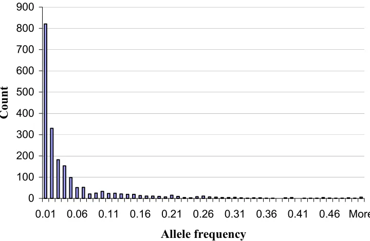
We surveyed 260 diverse maize inbred lines using 94 SSR loci. The inbreds can be roughly grouped as including 82 tropical lines, 35 temperate Stiff Stalk lines, 131 temperate non-Stiff Stalk lines, seven popcorn lines, and five sweet corn lines. The pedigrees for each line are too extensive to be reported here, but are available online (Supplemental Table S1). Among the lines, we detected a total of 2039 alleles or an average of 21.7 alleles per locus (Table 2.1). There is a large number of private alleles (556 or 27%) that are found in only one of the 260 inbred lines. Most alleles are in low frequency (Figure 2.1).

The number of alleles is not equivalent among loci. Loci with dinucleotide repeat motifs have considerably more alleles (average=23.9) than loci with repeat motifs of three nucleotides or larger (average=9.9; Table 2.1). This difference is also seen for genetic diversity, with dinucleotide SSRs (average=0.839) having a higher genetic diversity than longer-repeat SSRs (average=0.707). The mean genetic diversity of all SSRs is 0.818.

(33)

proportion of alleles at a locus that are simple multiples of the repeat motif length. For all 94 loci, the average stepwise mutation model index was 0.832 with dinucleotide SSRs (0.853) showing a higher index than other repeat loci (0.720).

The large number of alleles per locus and the common occurrence of private alleles suggest that a relatively small number of SSRs would be sufficient to uniquely fingerprint maize inbreds. For the 260 inbred lines that we sampled, the following six loci form a unique profile: bnlg244, bnlg2238, bnlg619, bnlg1191, bnlg1046 and dupssr28. Assuming the allele distribution of our inbred data is representative of all maize inbreds, the probability of sampling 260 independent lines without generating the same genotype for any two lines will be >0.99 by randomly selecting 10 loci. This number is nine if one only uses dinucleotide SSR and 12 if one uses longer-repeat SSR. Thus, very few SSRs are necessary if one wishes to uniquely fingerprint maize inbreds.

Genetic structure of inbred lines

We wished to assess the degree of relatedness among lines and to identify clusters of genetically similar lines. To do this, we used a model-based approach with the program STRUCTURE to subdivide the lines into clusters (Pritchard et al. 2000). Five sweet corn lines and seven popcorn lines were assigned to two pre-defined groups (Sweet and Popcorn) and were excluded in the STRUCTURE analysis. This was done because a pilot analysis showed that incorporating these 12 lines in the analysis interfered with the ability of STRUCTURE to converge on a robust solution. K(number of populations)

3

(34)

4

K = to 10 among runs of program. We used the run with highest log likelihood at

3

K = for the observed data to produce model-based groups (Table 2.2).

The model-based groups are largely consistent with known pedigrees of the lines (MMG and JSCS, pers. obs.). The largest group has 94 lines most of which are regarded by breeders as temperate non-stiff stalk lines (NSS). The next group has 58 lines most of which are either tropical or semitropical lines (TS). The smallest group has 33 lines, all of which are temperate stiff stalk lines (SS). The remaining 63 lines have less than 80% membership in any one group and were assigned to a mixed group. Supplemental Table S3 shows the proportional membership for these mixed lines in the three groups. Most mixed lines are either NSS-TS or NSS-SS mixtures. There are only four lines (Tzi16, Tzi25, Hi27, CML92) that present high membership of TS and SS.

STRUCTURE analysis was repeated to break the three main clusters into subclusters (Table 2.2). The SS group split into four subgroups, the TS group into five, and the NSS group seven subgroups. Supplemental Table S5 shows the proportional membership of the lines in the subgroups for the group to which they belong.

(35)

Genetic diversity within inbred groups

Gene diversity and mean numbers of alleles for the 94 SSRs were calculated for each group of inbreds (Table 2.1). The TS group is the most diverse with 13.49 alleles per locus and gene diversity of 0.81. NSS has less diversity than TS, which was revealed by the decreased allele number (12.84) and gene diversity (0.78). SS was found to be less diverse than NSS and TS. Our samples of Sweet and popcorn includes only a few lines, and thus, the small allele numbers in these groups were expected. In all groups, dinucleotide loci have a much larger allele number than longer-repeat loci. Gene diversity also shows a similar trend.

Maize inbreds show a high number of line-specific (556 or 27%) or group-specific (765 or 38%) alleles (Table 2.1). Far more line- and group-specific alleles are found in the TS group (204 and 305) than in the NSS group (121 and 173) despite a much smaller sample size for TS, indicating far greater diversity in tropical than in temperate inbreds.

(36)

Allelic richness of maize inbreds

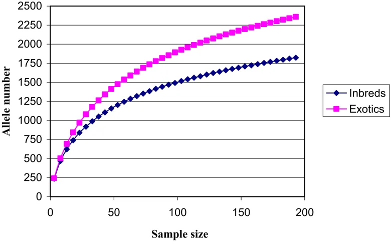
Comparison of diversity in inbreds to that in open pollinated landraces shows that the latter possess much greater diversity. For the exotics, the number of allele (2697 or 28.7 alleles per locus) and overall gene diversity (0.84) are higher than for the inbreds (2039 or 21.7; 0.82). To compare allelic richness in inbreds vs. landraces for equal sample sizes, we randomly selected equal numbers of samples from both germplasm pools (see Materials and Methods). This analysis reveals the greater allelic richness in exotics when the samples are equivalent (Figure 2.2). When the sample size is small (<20), the inbreds capture about 88% as many alleles as the exotics. When the sample size is large (>100), inbreds capture an about 78% as many alleles as the exotics.

(37)

Relationship of inbreds to exotic lines

To understand the relationship between the inbreds and exotics, we estimated the proportion of each inbred group's gene pool that was derived from four different segments of the exotics gene pool (Northern Flint, Southern Dent, Tropical Lowland and Tropical Highland). TS has its origin mostly from tropical lowland (66%) and tropical highland (18%) (Table 2.4). NSS and SS show very similar origins, being composed of roughly equal proportions of Northern Flint, Southern Dent and Tropical Lowland. Popcorn has a high proportion of Northern Flint germplasm (40%) with the rest of its genome coming mostly from Tropical Lowland (26%) and Southern Dents (23%). Sweet corn has the largest contribution from Northern Flint germplasm (72%). Overall, Tropical Highland maize has made a modest contribution to our set of inbreds than have the other three historical sources. Variances for these estimates are usually small (SD < 1%). Estimates of historical sources for individual inbreds are included in Supplemental Table S4.

Comparison of SSR and pedigree relationships

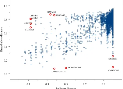
A Mantel test shows a highly significant (_p_<₁₀−6_{) correlation between pedigree and} SSR distance, although the correlation coefficient is relatively small (r=0.57). A plot of pedigree by SSR distances shows a general strong relationships but with many outliers (Figure 2.3).

(38)

We defined core sets of inbreds that capture the maximum number of alleles for a given sample size (Table 2.5). In selecting these sets, we constrained the selection to include six lines (A632, B37, B73, C103, Mo17, Oh43) of high agronomic importance. We also eliminated 8 lines (A654, B2, CM37, CMV3, CO109, I205, Q6199, R109B) because of poor agronomic quality under our field conditions. Additional core set of different sizes can be found in Supplemental Tables S5 and S6. Our study shows 10 lines can capture 28% of all the 2039 SSR alleles in the 260 lines, 20 lines capture 46% of the alleles, 30 lines capture 58%, and 50 lines capture 73%. In order to cover all the possible 2026 alleles, 193 lines were needed. The core sets generally include a large proportion of TS lines as expected since TS have the greatest allelic richness.

Linkage disequilibria

(39)

DISCUSSION SSR Diversity

Previous studies have shown that maize contains abundant SSRs (Senior et al. 1993a, 1993b, 1998) and that these SSRs are highly polymorphic even among small samples of maize inbreds (Chin et al. 1996; Taramino and Tingey 1996). These pioneering studies were conducted using relatively small numbers of inbreds (9 to 94) and loci (6 to 70). We have extended these earlier analyses by using both a large number of SSRs (94) and a much larger number of inbreds (260) that encompass a much greater portion of the maize gene pool. Our analyses uncovered abundant allelic variation with an average of 21.7 alleles per locus over 94 loci. This value greatly exceed the previously reported values of 5.21 (Senior et al. 1998), 6.6 (Taramino and Tingey (1996), 4.9 (Lu and Bernardo 2001), and 6.9 (Matsuoka et al. 2002) alleles per locus. The larger number of alleles observed in the present study can be attributed to the larger number of inbreds surveyed, the more diverse selection of inbreds (tropical, subtropical and temperate), and the inclusion of more dinucleotide repeat SSRs, which tend to be more polymorphic than SSRs with longer repeat motifs (Vigouroux et al. 2002).

(40)

more diverse set of inbred. If one considers only SSRs with trinucleotide or longer repeat motifs, then gene diversity in our sample (0.71) falls within the range of these previous reports.

We also showed that most maize SSRs generally fit a stepwise mutation model with 83% of the alleles fitting multiples of the length of the repeat motif of their respective loci. The 17% of alleles that deviate from the stepwise pattern likely represent cases where there have been indels in the regions flanking microsatellite repeat (Matsuoka et al.

2002a). The failure of these SSRs to fit exactly a stepwise model cautions against the use of models that assume a stepwise mutation process. In particular, estimates of genetic distance such as ₍_δµ₎2_{(Goldstein 1995) or measures of population subdivision based on} the stepwise mutation model (Slatkin 1995) would be inappropriate to apply to our data.

Genetic structure

(41)

We used the model-based approach of Pritchard et al. (2000) to define natural groups of maize inbreds. In performing this analysis, we discovered that the inclusion of small numbers of sweet (five) and popcorn (seven) lines in the analysis prevented the convergence to a robust solution. Apparently, these two groups were represented by too few lines to form distinct clusters, while at the same time they are too divergent from the other lines to fit into the clusters for those lines. Only when the sweet and popcorn lines were excluded did STRUCTURE converged on a robust solution with three clusters representing the temperate stiff stalks (SS), other temperate non-stiff stalks (NSS) lines, and tropical-subtropical (TS) lines. Thus, along with the predefined sweet and popcorn lines, we classify maize inbreds into five groups. Sixty-three lines did not fit into one of these five groups since they consist of a mixture of two or more of the primary groups. A comparison of genetic distances among the five groups indicates that SS are the most divergent (Table 2.3), a result consistent with the observation that the SS lines typically provide a strong heterotic response in crosses with other maize inbreds (Hallauer et al.

1988).

(42)

principally of Caribbean origin (Sriwatanapongse 1993), plus B96 from Maíz Amargo of Argentina. The CML-late subgroup is comprised of tropical lines tracing back to CIMMYT's late-maturing Tuxpeño composite populations. The CML-early subgroup contained lines derived from CIMMYT's early-maturing (in the tropics) Tuxpeño related materials and other intermediate-maturity sources. The NC subgroup consists of lines derived from Latin American tropical hybrids. Lines in the subgroup CML-P were largely derived from the La Posta Population 43 developed at CIMMYT from 16 lines of Tuxpeño origin (CIMMYT 1987).

(43)

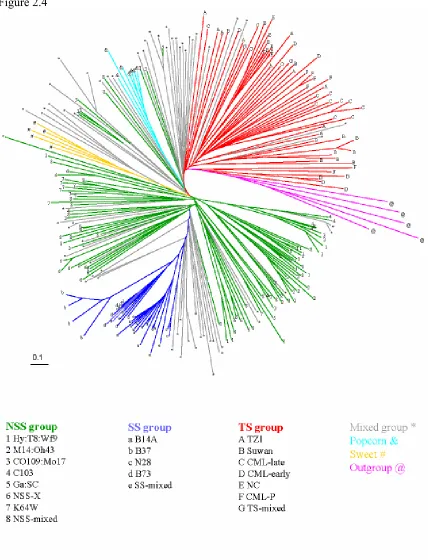
A Fitch-Margoliash tree based on the SSR data shows generally good agreement with the pedigree information and STRUCTURE analysis (Figure. 2.4, Supplemental Figure S1). There is a general separation of the TS, NSS and SS lines. Mixed lines are usually located between clusters of TS/NSS/SS lines. Within the SS lines, the four subgroups defined by the STRUCTURE analysis are perfectly matched with four clades. For the TS group, the tree has three clades that correspond to subgroups NC, Suwan, and CML-late. For the NSS lines, the tree has three clades that largely correspond to subgroups Hy:T8:Wf9, M14:Oh43 and K64W. All of the sweet corns fall in the same clade, as did all of the popcorns. The European (F2, F7, EP1) lines and one Canadian (CO255) line are closely grouped together, and this clade is neighbor to the sweet corn clade as expected since all these lines were derived from the Northern Flint landrace of the northern US and adjacent Canada (Galinat 1971; Doebley et al. 1985). NSS-X is also contained within a single large clade, despite the fact that these lines have heterogeneous pedigrees.

Genetic diversity among inbred groups

(44)

Five hundred and fifty-six of the 2039 alleles (27%) occur in only one inbred, and 765 alleles (38%) are restricted to a single model-based group of inbreds. These large proportions of private alleles are probably a function of the high mutation rate for maize SSRs (Vigouroux et al. 2002), allowing much new allelic variation to arise within lines after their initial development. This feature of maize SSRs contributes to their considerable discriminatory power, enabling one to fingerprint uniquely our entire set of 260 lines with as few as ten SSRs. This discriminatory power makes SSRs ideal markers for use in varietal identification (Smith et al. 1997) and for monitoring gene flow between lines (Dale et al. 2002). SSRs can also be used to determine pedigrees in maize inbreds and hybrids but more (e.g. 60 or more SSR loci ) are required to trace pedigrees than to provide for unique line identification especially when closely related inbreds are considered (Berry et al. 2002).

(45)

capture additional diversity by working with landrace accessions (Goodman 1985). It is likely that the landraces contain numerous agronomically useful alleles not represented in the inbreds and advanced populations with which breeders presently work.

Historical sources of maize inbreds

To better understand the relationship between our set of 260 inbreds and the broader maize germplasm pool from which they were derived, we made maximum likelihood estimates of the portions of four segments of the landrace gene pool (Northern Flint, Southern Dents, Tropical Lowland and Tropical Highland) represented in the five inbred groups. The results are consistent with historical records, pedigree information and geography. The temperate NSS and SS are composed of a near-equal mix of Tropical Lowland, Southern Dent and Northern Flints, although the Northern Flint portion is a bit smaller. Since Southern Dents themselves are thought to have been recently derived from tropical lowland germplasm (Galinat 1985; Doebley et al. 1988), the high portion of Tropical Lowland germplasm in NSS and SS lines likely represents a tropical contribution that came via the Southern Dents. The observation that NSS and SS are composed of only 25% Northern Flint is consistent with prior observations (Doebley et al.

1988).

(46)

to the possibility of using tropical highland germplasm to increase diversity within maize inbreds. The top four lines in terms of Northern Flint contribution (IA2132, IL14H, IL101t, P39) are all sweet corn. Some European lines (F2, F7) and one Canadian line (CO255) also have more than 50% Northern Flint origin. Va35, a southern US line, was found to have the largest Southern Dent proportion (63%).

Pedigree vs. genetic distance

Previous studies using molecular markers have generally shown a strong correlation between molecular marker and pedigree-based distance measures (Smith and Smith, 1992; Bernardo et al. 1997; Smith et al. 1997; Bernardo et al. 2000; Bernardo and Kahler 2001). Nonetheless, estimates of relatedness on the basis of pedigree data can differ from those based on molecular marker data (Bernardo et al. 2001). Calculations of relatedness based upon pedigree data are dependent upon the assumptions that both parents contribute an equal number of alleles, (i.e. no selection, mutation or genetic drift) and that the pedigree data are accurate. Another assumption is that founder genotypes (genotypes for which no further pedigree information on ancestors is available) are unrelated by pedigree. All of these assumptions can be violated.

(47)

than we did with our more diverse set of lines. Similarly, Bernardo et al. (2000) observed a correlation of 0.92 between SSR and pedigree using a small set of public inbreds with well-documented pedigrees. Our study also differs from these two prior studies in using a higher proportion of dinucleotide SSRs, which with their higher mutation rate, could weaken the correlation between SSR and pedigree distance.

Linkage disequilibrium

(48)

Perspective

(49)

ACKNOWLEDGEMENTS

(50)

REFERENCES

Anderson E, and Brown WL, Origin of Corn Belt maize and its genetic significance, pp. 124-148 in Heterosis - A record of researches directed toward explaining and utilizing the vigor of hybrids, edited by J. W. Gowen. Iowa State College Press, Ames, IA (1952).

Anonymous, MBS Genetics Handbook. Mike Brayton Seeds Inc., Ames, Iowa (1999). Austin DF, Lee M and Veldboom LR, Genetic mapping in maize with hybrid progeny

across testers and generations: plant height and flowering. Theor Appl Gen

102:163-176 (2001).

Bernardo R, Breeding potential of intra- and interheterotic group crosses in maize. Crop Science 41: 68-71 (2001)

Bernardo R, and Kahler K, North American study on essential derivation in maize: inbreds developed without and with selection from F2 populations. Theor. Appl. Genet 102: 986-992 (2001).

Bernardo R., Murigneux A, Maisonneuve JP, Johnsson C, and Karaman Z, RFLP-based estimates of parental contribution to F2- and BC1-derived maize inbreds. Theor. Appl. Genet. 94: 652-656. (1997)

Bernardo R, Romero-Severson J, Ziegle J, Hauser J, Joe L, Hookstra G, and Doerge R, Parental contribution and coefficient of coancestry among maize inbreds: pedigree, RFLP, and SSR data. Theor Appl Genet 100: 552-556 (2000).

(51)

Burr B, Burr FA, Thompson KH, Albertson MC and Stuber CW, Genetic mapping with recombinant inbreds in maize. Genetics 118:519-526 (1988).

Chin EC, Senior ML, Shu H and Smith JS, Maize simple repetitive DNA sequences: abundance and allele variation. Genome 39: 866-873 (1996).

Ching A, Caldwell KS, Jung M, Dolan M, Smith OS, Tingey S, Morgante M and Rafalski A, SNP frequency, haplotype structure and linkage disequilibrium in elite maize inbred lines. BMC Genet 3:19:1-14 (2002).

CIMMYT, CIMMYT report on maize improvement 1982-83, pp. 1-78. Centro Internacional de Mejoramiento de Maíz y Trigo, Chapingo, Mexico (1987).

Crosbie TM, Mock JJ and Pearce R, Inheritance of photosynthesis in a diallel among eight maize inbred lines from Iowa Stiff Stalk Synthetic. Euphytica 27:657-664 (1978).

Dale PJ, Clarke B and Fontes EMG, Potential for the environmental impact of transgenic crops. Nature Biotech. 20: 567-574 (2002).

Doebley J, Wendel JF, Smith JSC, Stuber CW and Goodman MM, The origin of cornbelt maize: the isozyme evidence. Econ. Bot. 42: 120-131 (1988).

Doebley J, Goodman MM and Stuber CW, Exceptional genetic divergence of the Northern Flint corns. Amer. J. Bot. 72: 64-69 (1986).

Edwards AWF, Likelihood: an account of the statistical concept of likelihood and its application to scientific inference. Cambridge University Press, Cambridge (1972). Edwards MD, Stuber CW and Wendel JF, Molecular-marker-facilitated investigations of

(52)

Excoffier L, Smouse P and Quattro J, Analysis of molecular variance inferred from metric distances among DNA haplotypes: Application to human mitochondrial DNA restriction data. Genetics 131: 479-491 (1992).

Felsenstein J, PHYLIP - Phylogeny Inference Package version 3.5c. Department of Genetics, University of Washington, Seattle (1993).

Fowler JE and Freeling M, Genetic analysis of mutations that alter cell fates in maize leaves: dominant Liguleless mutations. Developmental Genet. 18: 198-222 (1996). Galinat WC, The evolution of sweet corn. University of Massachusetts-Amherst College

of Agriculture Agricultural Experiment Station Research Bulletin 591: 1-20 (1971).

Galinat WC, Domestication and diffusion of maize, pp. 245-282 in Prehistoric Food Production in North America, edited by R. I. Ford. University of Michigan, Ann Arbor, MI (1985).

Gerdes JT, Behr CF, Coors JG and Tracy WF, Compilation of North American Maize Breeding Germplasm. Crop Sci. Soc. Am., Madison, Wisconsin. Pages: 1-202 (1993).

Goldstein DB, Ruiz Linares A, Cavalli-Sforza LL and Feldman MW, Genetic absolute dating based on microsatellites and the origin of modern humans. Proc. Natl. Acad. Sci. USA 92: 6723-6727 (1995).

Goodman MM, Exotic maize germplasm: Status, prospects, and remedies. Iowa State J. Res. 59: 497-529 (1985).

(53)

Goodman MM, Broadening the genetic diversity in breeding by use of exotic germplasm, pp. 139-148 in Genetics and Exploitation of Heterosis in Crops, edited by J. Liu et al. – page 30 G. Coors and S. Pandey. Crop Science Society of America, Madison, WI (1999).

Hallauer AR, Russell WA and Lamkey K, Corn breeding, pp. 463-564 in Corn and Corn improvement, edited by G. F. Sprague and J. W. Dudley. Crop Science Society of America, Madison, WI (1988).

Henry A and Damerval C, High rates of polymorphism and recombination at the

Opaque-2 locus in cultivated maize. Mol Gen Genet 256:147-157 (1997).

Kirkpatrick S, Gelatt CD and Vecchi MP, Optimization by simulated annealing. Science

220: 671-680 (1983).

Labate JKL, Mitchell S, Kresovich St, Sullivan H, Smith JSC, Molecular and historical aspects of corn belt dent diversity. Crop Sci 43: 80-91 (2003).

Liu K, Powermarker - A powerful software for marker data analysis. North Carolina State University Bioinformatics Research Center, Raleigh, North Carolina (www.powermarker.net) (2003).

Lu H and Bernardo R, Molecular marker diversity among current and historical maize inbreds. Theor Appl Genet 103: 613-617 (2001).

Malécot G, Les mathématiques de l'hérédité. Masson & Cie, Paris (1948).

Mantel N, The detection of disease clustering and a generalized regression approach.

(54)

Matsuoka Y, Mitchell SE, Kresovich S, Goodman MM, Doebley J, Microsatellites in Zea - variability, patterns of mutations, and use for evolutionary studies. Theor Appl Genet 104: 436-450 (2002a).

Matsuoka Y, Vigouroux Y, Goodman MM, Sanchez GJ, Buckler E et al., A single domestication for maize shown by multilocus microsatellite genotyping. Proc. Natl. Acad. Sci. USA 99: 6080-6084 (2002b).

Poethig RS, Heterochronic mutations affecting shoot development in maize. Genetics

119: 959-973 (1988).

Pritchard JK, Stephens M and Donnelly P, Inference of population structure using multilocus genotype data. Genetics 155: 945-959 (2000).

Remington DL, Thornsberry JM, Matsuoka Y, Wilson LM, Whitt SR et al., Structure of linkage disequilibrium and phenotypic associations in the maize genome. Proc. Natl. Acad. Sci. USA 98: 11479-11484 (2001).

Romero-Severson J, Smith JSC, Zeigle J, Hauser J, Joe L & Hookstra G. Pedigree analysis and haplotype sharing within diverse groups of Zea mays L. inbreds.

Theor. Appl. Genet., 103: 567-574 (2001).

Senior ML, and Heun M, Mapping maize microsatellites and polymerase chain reaction confirmation of the targeted repeats using a CT primer. Genome 36: 884-889 (1993).

(55)

Senior ML, Murphy JP, Goodman MM, Stuber CW, Utility of SSRs for determining genetic similarities and relationships in maize using an agarose gel system. Crop Sci 38: 1088-1098 (1998).

Slatkin M, A measure of population subdivision based on microsatellite allele frequencies.

Genetics 139: 457-462 (1995).

Smith JSC, Chin ECL, Shu H, Smith OS, Wall SJ, Senior ML, Mitchell SE, Kresovich S, Ziegle J, An evaluation of the utility of SSR loci as molecular markers in maize (Zea mays L): comparisons with data from RFLPS and pedigree. Theor Appl Genet 95: 163-173 (1997).

Smith OS, and Smith JSC, Measurement of genetic diversity among maize hybrids – a comparison of isozymic, RFLP, pedigree, and heterosis data. Maydica 37: 53-60 (1992).

Sriwatanapongse S, Jinahyon S and Vasal S, Suwan-1: maize from Thailand to the world, pp. 1-16. Centro Internacional de Mejoramiento de Maíz y Trigo, Chapingo Mexico (1993).

Taramino G and Tingey S, Simple sequence repeats for germplasm analysis and mapping in maize. Genome 39: 277-287 (1996).

Tenaillon MI, Sawkins MC, Long AD, Gaut RL, Doebley JF et al., Patterns of DNA sequence polymorphism along chromosome 1 of maize (Zea mays ssp. mays L.).

Proc. Natl. Acad. Sci. USA 98: 9161-9166 (2001).

(56)

Troyer AF, Chapter 14 - Temperate Corn. In Specialty Corn, A. Hallauer (ed.), CRC press (2001).

(57)

Table 2.1: Summary statistics for all inbreds and each subgroup

Statistics a Overall TS Sweet NSS Popcorn SS Mixed

Sample size 260 58 5 94 7 33 63

Alleles 2039 1268 272 1207 277 535 1321

Alleles per locus 21.7 13.49 2.89 12.84 2.95 5.69 14.05

Type I SSR alleles/locus 23.9 14.71 2.91 13.91 2.97 5.99 15.22 Type II SSR alleles/locus 9.9 7.07 2.80 7.20 2.80 4.13 7.93

Gene diversity 0.82 0.81 0.64 0.78 0.54 0.59 0.82

Type I SSR gene diversity 0.84 0.83 0.64 0.80 0.56 0.61 0.84 Type II SSR gene diversity 0.71 0.68 0.65 0.68 0.45 0.51 0.72

Group specific alleles 765 305 26 173 16 43 202

Group specific alleles/line 2.94 5.26 5.20 1.84 2.29 1.30 3.21 Group specific alleles (%) 24.05 9.56 14.33 5.78 8.04 15.29

Line specific alleles 556 204 18 121 11 36 166

Line specific alleles (%) 16.09 6.62 10.02 3.97 6.73 12.57

(58)

Table 2.2: List of the 260 lines by their model-based groupings Groupa Subgroupb Lines

Hy:T8:Wf9 CI21E, H49, Hy, Mo1W, Pa875, Pa880, T8, Va17, Va14, Va22, Va35, Va102, W64A, Wf9

M14:Oh43 A619, Gn2, H95, M14, Oh40B, Oh43, Oh43E, PA762, Va26, Va85 CO109:Mo17 A556, A682, CI.187-2, CO109, CO220, K187, Mo17, MS1334,

ND246, W401

C103 B57, C103, C123, DE2, L317, L1546, NC258, NC262 Ga:SC 4226, F44, Ga209, GT112, SC357, SC213R, SC213

NSS-X 38-11, A239, A659, AR4, CM7, CM37, R168, Mo44, MS71, NC260, PA884P, R4, R177, W22

K64W 33-16, CI.31A, CI.64, CI.66, CI.7, E2558W, Ky21, K55, K64, M162W NSS

NSS-mixed A554, A654, B2, B52, B70, B77, B97, B103, CO106, CO125, F6, Fe2, H99, Mt42, N6, Os420, Pa91, R109B, SD44, T234, W153R

B14A A214N, A632, A634, A635, A665, B14A, B64, B68, CM105, CM174, H91

B37 B37, B76, H84, NC250

N28 N28, N28Ht

B73 A679, A680, B73, B84, B104, B109, NC328, NC372, R229 SS

SS-mixed A641, De811, H100, N192, N196, NC294, NC368

TZI A6, CML52, CML238, CML287, NC358, Q6199, Tzi8, Tzi9, Tzi10, Tzi18

Suwan B96, CML69, CML228, CML349, Ki3, Ki9, Ki11, Ki14, Ki44, Ki2007 CML-late CML5, CML9, CML61, CML103, CML220, CML254, CML258,

CML261, CML264, CML314, Tx601

CML-early CML14, CML247, CML311, CML321, CML322, CML331, CML332 NC NC296, NC298, NC304, NC336, NC338, NC348, NC350, NC352,

NC354

CML-P CML10, CML11, CML45, CML277, CML281, CML333, CML341 TS

TS-mixed CML38, CML108, NC300, NC356 Sweet Ia2132, Il14H, Il101t, Il677a, P39

Popcorn HP301, I29, IDS28, IDS69, SA24, Sg18, Sg1533

Mixed A188, A272, A441-5, A656, B79, B94, B105, B164, C49A, CML77, CML91, CML92, CML218, CML323, CML328, CMV3, CO159, CO255, D940Y, DE3, EP1, F2, F2834T, F7, Hi27, I137TN, I205, IDT, Ki43, Ky226, Ky228, L578, Le23, Le773, M37W, Mo18W, Mo24W, Mp339, MS153, N7A, NC264, NC320, NC360, NC362, NC364, NC366, NC370, Oh7B, Oh603, SC55, SD40, SD46, T232, TEA, Tx303, Tzi11, Tzi16, Tzi25, U267Y, Va99, W117, W117Ht, W182B

(59)

any group. Seven popcorn lines and five sweet corn lines were assigned into predefined popcorn and sweet corn groups. Within TS, SS, and NSS group, an additional subclustering organizes each group into several distinct subgroups and one mixed subgroup by using the same scheme.

a_{The groups are SS - stiff stalk lines, NSS - non stiff stalk lines, TS -} tropical/semitropical lines, sweet corn, popcorn, and mixed lines (see text).

(60)

Table 2.3: Genetic distances between maize inbred groups

Group TS Sweet NSS Popcorn SS

TS - 0.58 0.29 0.52 0.47

Sweet 0.15 - 0.47 0.62 0.61 NSS 0.06 0.12 - 0.46 0.32

Popcorn 0.15 0.29 0.15 - 0.57

SS 0.18 0.28 0.14 0.31 -

(61)

Table 2.4: Historical sources for each maize inbred group

Group

Tropical Lowland (mean ± s.e.)

Southern Dents (mean ± s.e.)

Tropical Highland (mean ± s.e.)

Northern Flints (mean ± s.e.)

NSS 0.31±0.01 0.37±0.01 0.05±0.01 0.27±0.01

Popcorn 0.26±0.03 0.23±0.02 0.11±0.03 0.40±0.03

SS 0.32±0.01 0.38±0.01 0.08±0.01 0.23±0.01

Sweet 0.14±0.02 0.06±0.02 0.08±0.02 0.72±0.03

TS 0.66±0.01 0.11±0.01 0.18±0.01 0.04±0.01

(62)

Table 2.5: List of core sets of inbred lines Sample

size

Alleles obtained

Line list

10 579 A632, B37, B73, C103, Mo17, Oh43, CML5, Tzi18, CML91, CML52 20 943 A632, B37, B73, C103, Mo17, Oh43,, CML14, CML277, CML52, Tzi8,

M37W, CML281, CML228, Oh7B, Il14H, CML322, CML91, B96, Tx601, Mo18W

30 1179 A632, B37, B73, C103, Mo17, Oh43, B96, Tzi8, CML277, CML228, Ky21, Mo18W, Oh7B, CML5, CML322, CML220, A441-5, ML61, Tx303, CML14, CML91, CML311, CO159, CML281, Il101t, Tx601, CO255, A272, M37W, CML77

50 1481 A632, B37, B73, C103, Mo17, Oh43, CML77, CML261, IDS28,

CML277, B96, CML14, CML322, CML91, Mo18W, CML220, CML281, I137TN, Ky21, CML228, CML5, Tzi8, A272, A441-5, W401, Oh7B, CML349, CML69, Hi27, F2, CML61, P39, Tzi9, CML247, CI.7, CML254, NC364, CML328, Il14H, CO159, CML321, OS420, Va85, NC304, Tx303, CML311, NC348, M37W, B57, K55

(63)

Table 2.6: Percentage of SSR locus pairs in LD at a p=0.01level

Population No. of lines Observed % in LD Expected % in LDa

Overall 260 66.05%

NSS 94 19.29% 18.91%

TS 58 14.48% 9.13%

SS 33 28.92% 4.32%

(64)

FIGURE LEGENDS

Figure 2.1: Histogram of allele frequency. There are 2039 alleles in total. There is also a large number of the alleles (265 or 13%) that are at very low frequency (<0.01) although present in more than one inbred. One thousand-forty alleles (56%) are present at frequencies between 0.01 and 0.25, 72 alleles (3.5%) have frequencies between 0.25 and 0.50, 5 alleles (0.2%) have frequencies between 0.50 and 0.75, and only one allele (0.05%) has frequency above 0.75.

Figure 2.2: Plots of allele number obtained against sample size. For a given sample size, 1000 replicates were sampled from the inbreds dataset or exotics dataset without replacement and the genotypes were randomly broken into alleles. Then the mean number was calculated to give the plot from sample size 3 to 193. Log trendlines (not shown) fit the plots very well.

Figure 2.3: Plot of the proportion of shared SSR alleles distance between inbred lines by the pedigree distance between inbreds. Pedigree distance is defined as 1-Malecot Coefficient of Coancestry (Malecot 1948).

Figure 2.4: Fitch-Margoliash tree for the 260 inbred lines using the log transformed proportion of shared allele distance. The tree was rooted using five teosinte (Z. mays ssp.

(65)

Figure 2.1

0 100 200 300 400 500 600 700 800 900

0.01 0.06 0.11 0.16 0.21 0.26 0.31 0.36 0.41 0.46 More

Allele frequency

Coun

(66)

Figure 2.2

0 250 500 750 1000 1250 1500 1750 2000 2250 2500

0 50 100 150 200

Sample size

A

llele n

umb

er

(67)

Figure 2.3

0.1 0.3 0.5 0.7 0.9

Pedigree distance 0.0

0.2 0.4 0.6 0.8 1.0

Share

d al

le

dis

tance

CM37/CM7 AR4/B2

B2/FE2 AR4/FE2

B73/Tzi25

NC362/NC364 CM105/CM174

H84/Mt42 B37/Mt42

(68)

(69)

Chapter 3 Choosing Core Sets of Lines from a Large Germplasm Pool

Kejun Liu1, Xiang Yu1, and Spencer Muse1,2

1. Bioinformatics Research Center, North Carolina State University Raleigh, NC 27695

2. Correspondence: Dr Spencer V Muse

501 Partners II, Bioinformatics Research Center North Carolina State University

(70)

ABSTRACT

(71)

INTRODUCTION

There are a variety of settings where it is necessary to select a subset of lines, populations, or individuals to represent some larger set of germplasm. For instance, conservation geneticists may want to identify a “core set” of populations that maximize the total amount of genetic variation, subject to an upper limit on the number of lines they can maintain (Frankel 1984; Frankel and Brown 1984; Schoen and Brown 1983). Plant or animal breeders may wish to select a subset of available breeding lines or populations for breeding stock maintenance purposes (Brown 1989a; Gouesnard et al. 2000). Recognizing these objectives, Frankel and Brown (1984) defined a core set of lines as a subset of a larger germplasm collection that maximizes the possible genetic diversity with a minimum of repetitiveness. In this paper, we describe algorithms for selecting such a core set in a way that maximizes diversity for a given user-defined number of lines.

(72)

all the possible core sets of a given size, and then singles out the sets with the maximum total observed number of alleles at the surveyed loci. The key assumption of the M strategy is that observed allelic richness at the genotyped marker loci is correlated to the allelic richness at unobserved loci. Monte Carlo simulations of germplasm collections have shown that the M-strategy performs well under a variety of genetic models (Bataillon et al. 1996). The M-strategy is especially useful for inbreeding species because of the genome-wide correlation of genetic variation resulting from a decrease in the spatial decay of linkage disequilibrium (Schoen et al. 1993).

(73)

While this iterative search appears to be effective and provides an approximate solution to the core set selection problem, it does not guarantee an optimal solution. In fact, the nature of the algorithm’s swapping is likely to result in a local maximum rather than a global maximum. Furthermore, it is difficult to incorporate constraints on the composition of the core set collection under the Bataillon et al. strategy. In practice, it is often the case that a variety of constraints are placed on the final core set. As a simple example, suppose that the N lines in the germplasm collection have been stratified into several geographically distinct groups. It might be desirable to select a core set of k lines subject to the constraint that at least 3 lines from each geographic group are in the final set. It is not obvious how to incorporate such constraints in the Bataillon et al. algorithm. Below, we present an algorithm for finding constrained core sets that have globally maximum levels of a chosen genetic diversity measure.

(74)

METHODS

Given an existing germplasm collection of N lines with genetic polymorphism data, X, available, there are two prerequisites for choosing a subset, λ_k, of k lines to form a small, informative core set. First, an objective function, f(λ_k;X), must be chosen for measuring the information content of each subset. For the purpose illustrating the algorithms, we will use the total allele number of the subset as the objective function f (see Discussion for other useful measures). Having decided upon f, the goal is to find a subset of k lines,

λ*_k_{, that furnishes a maximum value of}_f_{from the set of all possible subsets of}_k_lines.

Exhaustive enumeration of all possible N

k

   



 k-subsets is infeasible for most applications.

For instance, with 50 lines, there are 1.2 × 1022_{possible core sets of size 12.}

Unconstrained Optimization

For the unconstrained case, a general simulated annealing algorithm was applied to choose a core set of lines. While the application of simulated annealing is straightforward in this setting, we outline it briefly in Appendix A to provide a framework for describing the solution to the constrained case.

Constrained Optimization

(75)

Suppose the germplasm collection is organized into several non-overlapping subsets, each falling into one of the four possible types: unconstrained, constrained, conserved, excluded. In our chosen core set we require all n_C lines from the conserved subset S_C, and none of the n_E lines from the excluded subset S_E. Lines from the unconstrained subset S_U may be included or excluded as needed. Each constrained subset,

S_i, i=1,2,...,m, has upper and lower bounds U_i and L_i, and the number of the n_i lines inS_i appearing in the final core set must fall between the bounds.

The challenging aspect of incorporating the constraints in a simulated annealing algorithm is producing a computationally efficient mechanism for exploring only valid core sets that satisfy all the constraints. In Appendix B we describe an algorithm for achieving this goal.

Multiple Selection Criteria

(76)

combination of criteria values for each line, much like the notion of a selection index in breeding settings. The value of this composite function then replaces the allelic richness value as our optimality criterion. Because different criteria have different ranges of possible values and follow different distributions, criteria should be normalized before the function is computed. If prior knowledge or theory provides appropriate normalization functions, they can be used. In the absence of such information, we take an empirical approach to the normalization process. A random sample of k-subsets is selected, and the values for each criterion are computed. The sample mean and standard deviation is then used to estimate the mean and standard deviation of the distribution for each criterion. The composite objective function is defined as w_j fj(λk;X)−µ ˆ j

ˆ

σ _j

j

∑

,

where w_j is the (user-provided) weight for jth criterion, f_j(λ_k;X) is the observed value of the chosen k-subset for the jth criterion, and ˆ µ _j and ˆ σ _j are the estimated means and standard deviations of the jth criteria from the random sampling process described above.

Program

(77)

RESULTS

Performance evaluations

We used a simple test data set to compare the performance of new and existing algorithms for selecting core sets. The test data set contains the 29 non stiff stalk inbred lines of maize from Matsuoka et al. (2002), each of which has been typed for 94 microsatellite markers (a larger set of 102 lines is used later in the Results section). We used total allele number as our objective function, and investigated the ability of methods to identify core sets varying in size from 2 to 10. The small number (29) of lines was chosen to allow for exhaustive evaluation of all possible core sets. In Table 3.1 we present a comparison of three different core set selection algorithms: (i) exhaustive search, (ii) the iterative search of Bataillon et al. (1996), and (iii) the simulated annealing algorithm of this paper. Simulated annealing was performed under a weak convergence condition (see Appendix A). The number of evaluations for each annealing schedule, R, was set to 100, and the cooling coefficient ρ was set to 0.8. Since the results of the simulated annealing and iterative searches rely on a random component, the values vary over replicate analyses of the same data. Thus, we report the means and standard deviations of the function values from 1000 replicate analyses of the 29 lines. To indicate the amount of time consumed by each method, we report for each method M, the total number of objective function evaluations required for a single replicate.

(78)

exhaustive search. In the worst case (k =2) the core set found by simulated annealing differed from the true maximum by an average of only 1.7, demonstrating that the algorithm on average recovers a core set within less than 1% of the true maximum value. For the most computationally challenging case ( k =10 ), the simulated annealing algorithm result is, on average, only 0.3% below the true value. In comparison, the average result of the Bataillon et al iterative algorithm falls more than 9% below the true maximum when k =10 . In no case did the Bataillon et al. approach outperform simulated annealing. Also important is the replicate-to-replicate variation of the core sets, described by the standard deviations from the 1000 replicate analyses. Note that simulated annealing has roughly half the variation of the Bataillon et al. method.

In the first column of Table 3.1 we see the rapid growth in evaluation number of the exhaustive search that necessitates the iterative and simulated annealing algorithms. Note that moving from core sets of size size 2 to core sets of size 10, the total evaluation number of the exhaustive search increases approximately 50,000-fold. In contrast, the evaluation number of simulated annealing increased only around 50%, while the Bataillon et al. algorithm showed an increase of 145%.

(79)

steps. The vertical axis in Figure 1 shows the percentage of replicate analyses in which the different methods achieved the true global maximum (found by exhaustive search). For example, when searching for a core set of 7 lines, simulated annealing with strong convergence conditions (R=500) evaluations reached the global maximum 100% of the time; using weak convergence conditions (R=100) the global maximum was found about 80% of the time. The Bataillon et al. algorithm found the global maximum in this case less than 20% of the time. In only one case did simulated annealing with strong convergence condition (R=500) evaluations fail to recover the true maximum at a rate greater than 95% (For the case of k =6, where multiple local maxima differ from the global maximum by only one allele). Simulated annealing outperformed the Bataillon et al. method in each case, with comparable computational expense (The number of core set evaluations for iterative search is larger than that of the simulated annealing with

100

R= but less than that of the simulated annealing with R=500)

(80)

Improving performance with weighted sampling

In the algorithms described in Appendices A and B, we do not specifically describe the random sampling procedure we use to select lines from the available set. In the simple case, we sample lines uniformly. Efficiency can be improved by selecting lines from the available set according to a non-uniform distribution. The use of a weighted sampling scheme will not change the behavior of global convergence, but can improve the convergence speed significantly. The weights associated with each line are dependent on the specific criterion function, but should be assigned in way that more promising core sets will get evaluated with higher probability. When the objective is to maximize the total allele number of the core set, we have found that weights for each line based on the private allele number prove to be effective (the private allele number for a line is simply the number of alleles present only in that line). Private alleles will always increase the total allele number, so lines with many private alleles are preferred. Similar weighting schemes can be developed for other criteria.

Selecting a core set of maize inbreds

(81)

(82)

DISCUSSION

The simulated annealing algorithm developed in this paper has been shown to be a more effective and efficient means for selecting core sets of lines than existing published methods. This result is perhaps not surprising, given the versatility of simulated annealing in providing effective solutions to hard combinatorial optimization problems (Kirkpatrick

et al. 1983; Goradia and Lange 1988; Lukashin et al. 1992). An important practical decision in the use of this algorithm, or, indeed, in the use of any algorithm for selecting core sets based on genetic data, is the choice of a measure describing core set quality. We used total allele number for illustrative purposes in this paper, but other measures may be more appropriate in some settings. For example, one might want to include allele frequency information if the inclusion of rare alleles is not of particular value. In this case, the use of allelic diversity as a criterion considering both allele number and frequency would be a superior choice. An advantage of the simulated annealing method is the ease of incorporating non-genetic data into the selection criteria. Care must be taken when combining these data types, and normalization procedures are imperative. Our work suggests that simple adjustments based on forming “z-scores” from the normal distribution are usually sufficient. However, it is advisable to carry out empirical experiments investigating randomly chosen core sets to check for substantial deviations from normality.

The computational problem addressed in this work is an example of the minimum test set

(83)

(84)

ACKNOWLEDGEMENTS