The Entropy of Words—Learnability and Expressivity across More Than 1000 Languages

(1)

Article

The Entropy of Words—Learnability and Expressivity

across More Than 1000 Languages

Christian Bentz1,2*, Dimitrios Alikaniotis3, Michael Cysouw4and Ramon Ferrer-i-Cancho5

1 _{DFG Center for Advanced Studies, University of Tübingen, Rümelinstraße 23, D-72070 Tübingen,}

Germany; [email protected]

2 _{Department of General Linguistics, University of Tübingen, Wilhemstraße 19-23, D-72074 Tübingen,}

Germany

3 _{Department of Theoretical and Applied Linguistics, University of Cambridge, Cambridge, United}

Kingdom

4 _{Forschungszentrum Deutscher Sprachatlas, Philipps-Universität Marburg, Pilgrimstein 16, D-35032}

Marburg

5 _{Complexity and Quantitative Linguistics Lab, LARCA Research Group, Departament de Ciències de la}

Computació, Universitat Politècnica de Catalunya, Barcelona, Catalonia, Spain

* Correspondence: [email protected]

Abstract: The choice associated with words is a fundamental property of natural languages. It lies at the heart of quantitative linguistics, computational linguistics, and language sciences more generally. Information-theory gives us tools at hand to measure precisely the average amount of choice associated with words – the word entropy. Here we use three parallel corpora – encompassing ca. 450 million words in 1916 texts and 1259 languages – to tackle some of the major conceptual and practical problems of word entropy estimation: dependence on text size, register, style and estimation method, as well as non-independence of words in co-text. We present three main results: 1) a text size of 50K tokens is sufficient for word entropies to stabilize throughout the text, 2) across languages of the world, word entropies display a unimodal distribution that is skewed to the right. This suggests that there is a trade-off between the learnability and expressivity of words across languages of the world. 3) There is a strong linear relationship between unigram entropies and entropy rates, suggesting that they are inherently linked. We discuss the implications of these results for studying the diversity and evolution of languages from an information-theoretic point of view.

Keywords: natural language entropy; entropy rate; unigram entropy; quantitative language typology

1. Introduction

Symbols are the building blocks of information. When concatenated to strings, they give rise to surprisal and uncertainty – as a consequence of choice. This is the fundamental concept underlying information encoding. Natural languages are communicative systems harnessing this information encoding potential. Their fundamental building blocks are words. For any natural language, the average amount of information a word can carry is a basic property, an information-theoretic fingerprint that reflects its idiosyncrasies, and sets it apart from other languages across the world. Shannon [1] defined theentropy– oraverage information content– as a measure for the choice associated with symbols in strings. Since Shannon’s [2] original proposal, many researchers have undertaken great efforts to estimate the entropy of written English with highest possible precision [3–6], and to broaden the account to other natural languages [7–11].

Entropic measures in general are relevant for a wide variety of linguistic and computational subfields. For example, several recent studies engage in establishing information-theoretic and corpus-based methods for linguistic typology, i.e. classifying and comparing languages according to their information encoding potential [10,12–16], and how this potential evolves over time [17–19]. Similar methods have been applied to compare and distinguish non-linguistic sequences from written

Preprints (www.preprints.org) | NOT PEER-REVIEWED | Posted: 27 April 2017 doi:10.20944/preprints201704.0180.v1

(2)

2 of 34

language [20,21], though it is controversial whether this helps with more fine-grained distinctions between symbolic systems and written language [22,23].

In the context of quantitative linguistics, entropic measures are used to understand laws in natural languages, such as the relationship between word frequency, predictability and the length of words [24–27], or the trade-off between word structure and sentence structure [10,13,28]. Information-theory can further help to understand the complexities involved when building words from the smallest meaningful units, i.e. morphemes [29,30].

Beyond morphemes and word forms, the surprisal of words in co-text is argued to be related to syntactic expectations [31]. For instance, the usage of complementizers such as “that” might serve to smooth over maxima in the information density of sentences [32]. This has become known as the

Uniform Information Density(UID) hypothesis. It was introduced in the 1980s by August and Gertraud Fenk [33], and developed in a series of articles (see [34] and references therein). For a critical review of some problematic aspects of the UID hypothesis see [35] and [36].

In optimization models of communication, word entropy is a measure of cognitive cost [37]. These models shed light on the origins of Zipf’s law for word frequencies [38,39] and a vocabulary learning bias [40]. With respect to the UID hypothesis, these models have the virtue of defining explicitly a cost function and linking the statistical regularities with the minimization of that cost function.

Finally, in natural language processing, entropy (and related measures) have been widely applied to tackle problems relating to machine translation [41,42], distributional semantics [43–46], information retrieval [47–49], and multiword expressions [50,51].

All these accounts crucially hinge upon estimating the probability and uncertainty associated with different levels of information encoding in natural languages. Here we focus on theword entropy

of a given text and language. There are two central questions associated with this measure: 1) what is the text size (in number of tokens) at which word entropies reach stable values? 2) How much systematic difference do we find across different texts and languages? The first question is related to the problem of data sparsity. The minimum text size at which results are still reliable is a lower bound on any word entropy analysis. The second question relates to the diversity that we find across languages of the world. From the perspective of linguistic typology, we want to understand and explain this diversity.

In this study, we use state-of-the-art methods to estimate both unigram entropies [52] (for a definition see Section 3.2.4), and theentropy rateper word according to Gaoet al.[5] (Section3.2.5). Unigram entropy is the average information content of words assuming that they areindependent of the co-text. The entropy rate can be seen – under certain conditions (see Section3.2.5) – as the average information content of words assuming that theydepend on a sufficiently long, preceding co-text. For both measures we first establish stabilization points for big parallel texts in 21 languages. Based on these stabilization points, we select texts with sufficiently large token counts from a massively parallel corpus and estimate word entropies across more than 1000 texts and languages. Our analyses illustrate three major points:

1. Both unigram entropies and entropy rates reach stable values at around 50-100K word tokens across different languages. Hence, we do not need massive corpora to meaningfully compare languages with regards to their word entropies – as long as we keep the content of texts constant (Section5.1).

2. Across languages of the world, unigram entropies display a unimodal distribution around a mean of ca. 9 bits/word, with a standard deviation of ca. 1 bit/word. Entropy rates display a unimodal distribution around a mean of ca. 6 bits/word, with a standard deviation of ca. 1 bit/word. In both cases, the distribution is skewed to the right. Hence, there seems to be a strong pressure to keep the mass of languages in a relatively narrow entropy range, especially for the difference between unigram entropy and entropy rate (Section 5.2). This is in line with earlier findings [8,9]. There are no languages with a unigram entropy of less

(3)

3 of 34

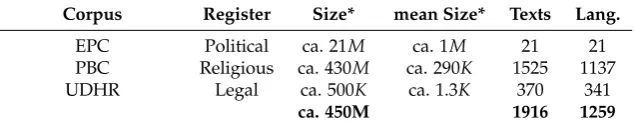
Table 1. Information on the parallel corpora used.

Corpus Register Size* mean Size* Texts Lang.

EPC Political ca. 21M ca. 1M 21 21

PBC Religious ca. 430M ca. 290K 1525 1137

UDHR Legal ca. 500K ca. 1.3K 370 341

ca. 450M 1916 1259

*in number of tokens

than 6 bits/word (if estimated based on 50K tokens). This observation is in agreement with optimization models of communication, where entropy is regarded as a cost to minimize in conflict with mutual information maximization. Zipf’s law for word frequencies emerges in a critical balance between these two forces [39]. We further argue that this trade-off reflects two basic pressures on natural communication systems:learnabilityvs.expressivity.

3. There is a strong positive linear relationship between unigram entropies and entropy rates (r= 0.96,p < 0.0001). This allows us to formulate a simple linear model that predicts one from the other (Section5.3). Given that unigram entropy estimation is computationally much more efficient than entropy rate estimation, this finding can help to reduce computational costs.

Finally, we argue that information theoretic properties like word entropy are not only relevant for computational linguistics and quantitative linguistics, but that they constitute a basic property of human languages. Understanding and modelling the differences and similarities in the information that words can carry is an undertaking at the heart of language sciences more generally.

2. Data

To estimate the entropy of words, we first need a comparable sample of texts across many languages. Ideally, the texts should have the same content, as differences in registers and style can interfere with the range of word forms used, and hence the entropy of words [53]. To control for constant content across languages, we use three sets of parallel texts: 1) theEuropean Parliament Corpus(EPC) [54], 2) theParallel Bible Corpus(PBC) [55],1and theUniversal Declaration of Human Rights

(http://www.unicode.org/udhr/). Details about the corpora can be seen in Table 1. The general advantage of the EPC is that it is big in terms of numbers of word tokens per language (ca. 30M),2 whereas the PBC and the UDHR are smaller (ca. 290K and 1.3K word tokens per language). However, the PBC and UDHR are massively parallel in terms of encompassing more than 1000, and more than 300 languages respectively. These are numbers of texts and languages that we actually used for our analyses. The raw corpora are bigger. However, some texts and languages had to be excluded due to their small size, or due to pre-processing errors (see Section3.1).

3. Theory

3.1. Word types and tokens

The basic information encoding unit chosen in this study is the word.3 Aword type is here defined as a unique string of alphanumeric UTF-8 characters delimited by white spaces. All letters are converted to lower case and punctuation is removed. Aword tokenis then any reoccurrence of a word type. For example, the pre-processed first verse of theBook of Genesisin English reads:

1 _{Last accessed on 02/06/2016}

2 _{Though we only use around 1M tokens for each language, since this is enough for the stabilization analyses.} 3 _{Note that earlier studies on the entropy of English [}₂_,₄_,₆_{] often chose characters instead.}

(4)

4 of 34

in the beginning god created the heavens and the earth and the earth was waste and empty [...]

The set of word types (in lower case) for this sentence is

V={in,the,beginning,god,created,heavens,and,earth,was,waste,empty}. (1) Hence, the number of word types in this sentence is 11, but the number of word tokens is 17, sincethe,and, andearthoccur several times. Note that some scripts, e.g. those of Mandarin Chinese (cmn) and Khmer (khm), delimit phrases and sentences by white spaces, rather than words. Such scripts have to be excluded for the simple word processing we propose. However, they constitute a negligible proportion of our sample (≈0.01%). In fact, ca. 90% of the texts are written in Latin-based script. For more details and caveats of text pre-processing see AppendixA.

Though definitions of “word-hood” based on orthography are taken as a given in most corpus and computational linguistic studies, they are not necessarily uncontroversial from a linguistically more informed point of view. Haspelmath [56] and Wray [57] point out that there is a whole range of orthographic, phonetic and distributional definitions for the concept “word”, which can yield different results for specific cases. However, a recent study on compression properties of parallel texts vindicates the usage of orthographic words as information encoding units, as it shows that these are optimal-sized for describing the regularities in languages [58].

Hence, we suggest to start with the orthographic word definition based on non-alphanumeric characters in written texts. Not the least because it is a computationally feasible strategy across many hundreds of languages. Our results might then be tested against more fine-grained definitions, as long as these can be systematically applied to language production data.

3.2. Word entropy estimation

A crucial pre-requisite for entropy estimation is the approximation of the probabilities of word types. In a text, each word typewi has a token frequency fi = f req(wi). Take the first verse of the

English Bible again.

in the beginning god created the heavens and the earth and the earth was waste and empty [...]

In this example, the word typetheoccurs 4 times,andoccurs 3 times, etc. As a simple approximation,

p(wi)can be estimated via the so-calledmaximum likelihoodmethod [59]:

ˆ

p(wi) =

fi

∑V j=1fj

, (2)

where the denominator is the overall number of word tokens. We thus have probabilities of ˆp(the) = 4

17, ˆp(and) = 3 17, etc.

Assume a text is a random variableTcreated by a process of drawing (with replacement) and concatenating tokens from a set (or vocabulary) of word typesV ={w1,w2, ...,wV}, with vocabulary

sizeV=|V |, and a probability mass functionp(w) =Pr{T=w}forw∈ V. Given these definitions, the theoretical entropy ofTcan be calculated as [60]

H(T) =−

V

∑

i=1

p(wi)log2p(wi). (3)

In this case,H(T)can be seen as theaverage information contentof word types. A crucial step towards estimatingH(T)is to reliably approximate the probabilities of word typesp(wi).

(5)

5 of 34

The simplest way to estimateH(T) is the maximum likelihood estimator – also calledplug-in

estimator – which is obtained replacing p(w)by ˆp(w)(Eq. 2). For instance, our example “corpus” yields:

ˆ

H(T) =−

4 17log2

4 17

+ 3

17log2

3 17

+. . .+ 1 17log2

1 17

≈3.2bits/word. (4)

Notice an important detail: we have assumed that p(wi) = pˆ(wi) = 0 for all the types that have

not appeared in our sample. Although our sample did not contain "never", the probability of "never" in an English text is not zero. We have also assumed that the relative frequency of the words that have appeared in our sample is a good estimation of their true probability. Given the small size of our sample, this is unlikely to be the case. The bottom line is that for small text sizes we will underestimate the word entropy using the maximum likelihood approach [61,62]. A range of more advanced entropy estimators have been proposed to overcome this limitation [6,52,59,63]. These are outlined in more detail in AppendixB, and tested with our parallel corpus data.

The conditions (e.g. the sample size) under which the entropy of a source can be estimated reliably are a living field of research ([64] and references therein). Proper estimation of entropy requires that certain conditions are met. Stationarity and ergodicity are typically named as such4(e.g., [63,64]). Another condition is finiteness (a finite set of types). While stationarity and ergodicity tend to be presented and discussed together in research articles, finiteness is normally stated separately, typically as part of the initial setting of the problem (e.g., [63,64]). A fourth usual condition is the assumption that types are independent and identically distributed (i.i.d.) [61,63,64]. Hence, for proper entropy estimation the typical requirements are either (a) finiteness, stationarity and ergodicity, or (b) only finiteness and i.i.d., as stationarity and ergodicity follow trivially from the i.i.d. assumption. In the following, we review two problems relating to the stationarity and the i.i.d. assumptions.

3.2.1. Problem 1: The infinite productive potential of languages

The first problem relates to the productive potential of languages. In fact, it is downright impossible to capture the actual repertoire of word types. Even if we captured the whole set of linguistic interactions of a speaker population in a corpus, we would still not capture the productive potential of the language beyond the finite set of linguistic interactions.

Theoretically speaking, it is always possible to expand the vocabulary of a language by compounding (recombining word types to form new word types), affixation (adding affixes to existing words), or by creating neologisms. This can be seen in parallel to Chomsky’s [65][p.8] reappraisal of Humboldt’s “make infinite use of finite means” in syntax. The practical consequence is that even for massive corpora like the British National Corpus, vocabulary growth is apparently not coming to a halt [66–68]. Thus, we never actually sample the whole set of word types of a language. However, the concentration of tokens on a core vocabulary [67,69] potentially alleviates this problem. Still, word entropy estimation is a harder problem than entropy estimation for characters or phonemes types, since the latter have a repertoire that is finite and usually small.

3.2.2. Problem 2: Short- and long-range correlations between words

In natural languages, we find co-occurrence patterns implying that word types in a text sequence are not independent events. This is the case for collocations, namely blocks of consecutive words that behave as a whole. Examples include place names such as "New York" or fixed expressions such

4 _{Stationarity means that the statistical properties of blocks of words of some length do not depend on their position in}

the text sequence. Ergodicity means that statistical properties of a sufficiently long text sequence matches the average properties of the ensemble of all possible text sequences.

(6)

6 of 34

as "kith and kin", but also many others that are less obvious. They can be detected with methods determining if some consecutive words co-occur with a frequency that is greater than expected by chance [70]. Collocations are examples ofshort-range correlationsin text sequences. Text sequences also exhibitlong-range correlations, i.e. correlations between types that are far away in the text [8,71]. 3.2.3. Our perspective

We are fully aware of both Problem 1 and 2 when estimating the word type entropy of real texts, and the languages represented by them. However, our question is not so much: what is the exact entropy of a text or language? but rather: how precisely do we have to approximate it to make a meaningful cross-linguistic comparison possible? To address this practical question, we need to establish the number of word tokens at which estimated entropies reach stable values – given a threshold of our choice. Furthermore, we incorporate entropic measures which are less demanding in terms of assumptions. Namely, we includeh, the entropy rate of a source, as it does not rely on the i.i.d. assumption. We elaborate onhin the next two subsections.

3.2.4.n-gram entropies

When estimating entropy according to Equation3, we assumeunigrams, i.e. single, independent word tokens, as “blocks” of information encoding. As noted above, this assumption is generally not met for natural languages. To incorporate dependencies between words, we could usebigrams,

trigrams, or more generallyn-gramsof any size, and thus capture short- and long-range correlations by increasing “block” sizes to 2, 3, n. This yields what are variously calledn-gramorblock entropies[6] defined as

Hn(T) =−

Vn

∑

i=1

p(wi,wi+1, ...,wn)× log2p(wi,wi+1, ...,wn), (5)

where n is the block size, and Vn is the “alphabet” of n-grams. However, since the number of

differentn-grams grows exponentially withn, very big corpora are needed to get reliable estimates. Schürmann & Grassberger [6] use an English corpus of 70M words, and assert that entropy estimation beyond a block size of 5 characters (not words) is already unreliable. Our strategy is to stick with block sizes of 1, i.e.unigram entropies. However, we implement a more parsimonious approach to take into account long-range correlations between words along the lines of earlier studies by Montemurro and Zanette [8,9].

3.2.5. Entropy rate

Instead of calculatingHn(T)with ever increasing block sizesn, we use an approach focusing on

a particular feature of the entropy growth curve: the so-calledentropy rate, orper-symbol entropy[5]. In general, it is defined as the rate at which the word entropy grows as the number of word tokensN

increases [72, p.74], i.e.

h(T) = lim

N→∞ =

1

NHn(T) (6)

= 1

NH(t1,t2, ...,tN), (7)

wheret1,t2, ...,tNis a block of consecutive tokens of lengthN. Given stationarity, this is equivalent to

[72, p.75]

h(T) = lim

N→∞H(tN|t1,t2, ...,tN−1). (8)

In other words, as the number of tokens N approaches infinity, the entropy rate h(T) reflects the average information content of a tokentNconditioned onallpreceding tokens. Soh(T)accounts for

all statistical dependenciesbetween tokens [63]. Note that in the limit, i.e. as block sizenapproaches

(7)

7 of 34

infinity, the block entropy per token converges to the entropy rate. Also, for an independent and identically distributed (i.i.d) random variable, the block entropy of block size 1, i.e. H1(T), is identical to the entropy rate [63]. However, as pointed out above, in natural languages words are not independently distributed.

Kontoyiannis et al. [4] and Gao et al. [5] apply findings on optimal compression by Ziv & Lempel [73,74] to estimate the entropy rate. More precisely, Gao et al. [5] show that entropy rate estimation based on the so-calledincreasing window estimator, or LZ78 estimator [72], is efficient in terms of convergence. The conditions for this estimator are stationarity and ergodicity of the process that generates a textT.

Applied to the problem of estimating word entropies, the method works as follows: for any given word tokentifind the longest match-lengthLifor which the token stringsi_i+l−1= (ti,ti+1, ...,ti+l−1) matches a preceding token string of the same length in(t1, ...,ti−1). Formally, we defineLias

Li=1+max{0≤l ≤i:sii+l−1=s j+l−1

j for some 0≤j≤i−1}. (9)

This is an adaptation of Gao et al.’s [5] match-length definition.5 To illustrate this, take the example from above again:

in₁ the₂ beginning₃ god₄ created₅ the₆ heavens₇ and₈ the₉ earth₁₀ and₁₁ the₁₂

earth₁₃ was₁₄ waste₁₅ and₁₆ empty₁₇ [...]

For the word tokenbeginning, in positioni =3, there is no match in the preceding token string (in the). Hence, the match-length isl3= 0(+1) =1. In contrast, if we look atandin positioni=11, then the longest matching token string isand the earth. Hence, the match-length isl11 =3(+1) =4.

Note that the average match-lengths across all word tokens reflect theredundancy in the token string – which is the inverse ofunpredictability orchoice. Based on this connection, Gao et al. [5] (Equation 6) show that the entropy rate of a text can be approximated as

ˆ

h(T) = 1

N

∑

i=2 log₂i

Li

, (10)

whereNis the overall number of tokens, andiis the position in the string. Here we approximate the entropy rateh(T)based on a textTas ˆh(T)given in Equation10.

4. Methods

We estimateunigram entropies– i.e. entropies for block sizes of 1 (H1(T)) – with nine different estimation methods, using the R package entropy [75], and the Python implementation of the

Nemenman-Shafee-Bialek(NSB) [52] estimator. For further analyses, we especially focus on the NSB estimator, as it has been shown to have a faster convergence rate compared to other block entropy estimators [59].6 Moreover, we implemented the entropy rate estimator ˆh(T)as in Gao et al.’s [5] proposal in both Python andR, available ongithub.7 This was inspired by an earlier implementation by Montemurro & Zanette [8] of Kontoyiannis et al.’s [4] estimator.

As one estimates entropy with increasingly longer “prefixes” (i.e. runs of text preceding a given token), a fundamental milestone is convergence, namely, the prefix length at which the true value is reached with an error that can be neglected. However, the “true” entropy of a productive system like natural language is not known. For this reason, we replace convergence by another important

5 _{Note that Gao et al. [}₅_{] give a more general definition that also holds for the so-called}_{sliding window}_{, or}_LZ77_estimator. 6 _{https://gist.github.com/shhong/1021654/}

7 _{https://github.com/dimalik/EntropyEstimator}

(8)

8 of 34

milestone: the number of tokens at which the next 10 estimations of entropy have a SD (standard deviation) that is sufficiently small, e.g., below a certain threshold (α = 0.1). If L is the number

of tokens, SD is defined as the standard deviation that is calculated over entropies obtained with prefixes of lengths

L,L+1K,L+2K, ...,L+10K. (11)

Krepresents the number 1000 here. We say that entropies have stabilized when SD< α, whereαis

the threshold. Notice that this is indeed a local stabilization criterion. Here we chooseLto run from 1Kto 90K. We thus get 90 SD values per language. The threshold isα=0.1. The same methodology

is used to determine when the entropy rate has stabilized.

Note that both [8] and [10] use a more coarse-grained stabilization criterion. Namely, in [8] entropies are estimated for two halves of each text, and then compared to the entropy of the full text. Only texts with a maximum discrepancy of 10% are included for further analyses. Similarly, [10] compares entropies for the first 50% of the data and for the full data. Again, only texts with a discrepancy of less then 10% are included. In contrast, [11] establishes the convergence properties of different off-the-shelf compressors by estimating the encoding rate with growing text sizes. This has the advantage of giving a more fine-grained impression of convergence properties. Our assessment of entropy stabilization follows a similar rationale, though with words as information encoding units, rather than characters, and with our own implementation of Gao et al.’s entropy estimator rather than off-the-shelf compressors.

5. Results

We first assess the minimum text sizes at which bothunigram entropiesandentropy ratesstabilize, i.e. SD<0.1, using a subset of 21 languages (Section5.1) of the European Parliament Corpus (EPC). The EPC was chosen for this task since it is the largest in terms of number of tokens, ranging up to several millions. We then select texts from the full Parallel Bible Corpus (PBC) which have enough tokens, estimate their entropies, and compare their spread on an entropy spectrum (Section5.2). The

Universal Declaration of Human Rights(UDHR) is used in Appendix Dand AppendixFto illustrate that there are strong correlations between unigram entropies for different estimators and different corpora. Finally, in Section5.3, we investigate the correlation and linear relationship betweenunigram entropiesandentropy rates.

5.1. Entropy stabilization throughout the text sequence

5.1.1. Unigram entropies

Figure 1 illustrates the stabilization of unigram entropies (H1(T)) across 21 languages of the EPC. Nine different entropy estimators are used here, including the simple maximum likelihood estimator (ML). The estimation methods are further detailed in AppendixB. Some slight differences between estimators are visible. For instance, Bayesian estimation with a Laplace prior (Lap) yields systematically higher results compared to the other estimators. However, this difference is in the decimal range. If we take the first panel with Bulgarian (bg) as an example: at 100K tokens, the lowest estimated entropy value is found for maximum likelihood estimation ( ˆHML₌_{10.11), whereas}

the highest values are obtained for Bayesian estimation with Laplace and Jeffrey’s priors respectively ( ˆHLap = 10.66 and ˆHLap = 10.41). This reflects the expected underestimation-bias of the ML estimator, and the overestimation-biases of the Laplace and Jeffrey’s priors, which have been reported in an earlier study [59].

However, overall the stabilization behaviour of entropy estimators is similar across all languages. Namely, in the range of ca. 0 to 25K tokens, they all undergo a fast growth, and start to stabilize after 25K. This stabilization behaviour is visualized in Figure2. Here, standard deviations of estimated entropy values (y-axis) are plotted against text sizes in number of tokens (x-axis). A

(9)

9 of 34

standard deviation of 0.1 is given as a reference line (dashed grey). Across the 21 languages, SDs fall below this line at 50K tokens at the latest.

Remember that – relating toProblem 1– we were asking for the text size at which a meaningful cross-linguistic comparison of word entropies is possible. We can give a pragmatic answer to this question: If we want to estimate the unigram entropy of a given text and language with a local

precision of one decimal place after the comma, we have to supply >50K tokens. We use the term

localto emphasize that this is not precision with respect to the true entropic measure, but with respect to prefixes of a length within a certain window (recall Section4).

Furthermore, note that the curves of different estimation methods in both Figure1and 2have similar shapes, and, in some cases, are largely parallel . This suggests that despite the methodological differences, the values are strongly correlated. This is indeed the case. In fact, even the results of the simple ML method are strongly correlated with the results of all other methods, with Pearson’sr

ranging from 0.94 to 1. See AppendixDfor details.

(10)

10

of

34

Polish (pl) Portuguese (pt) Romanian (ro) Slovak (sk) Slovene (sl) Spanish (es) Swedish (sv) French (fr) German (de) Hungarian (hu) Italian (it) Latvian (lv) Lithuanian (lt) Modern Greek (el) Bulgarian (bg) Czech (cs) Danish (da) Dutch (nl) English (en) Estonian (et) Finnish (fi)

0 25000 50000 75000 100000 0 25000 50000 75000 100000 0 25000 50000 75000 100000 0 25000 50000 75000 100000 0 25000 50000 75000 100000 0 25000 50000 75000 100000 0 25000 50000 75000 100000

8 10 12

Number of Word Tokens

Estimated Entrop

y (bits/w

ord)

Method

CS

Jeff

Lap

minimax

ML

MM

NSB

SG

Shrink

Figure 1. Unigram entropies (y-axis) as a function of text length (x-axis) across 21 languages of the EPC corpus. Unigram entropies are estimated on prefixes of the text sequence increasing by 1K tokens. Thus, the first prefix covers tokens 1 to 1K, the second prefix covers tokens 1 to 2K, etc. The number of tokens is limited to 100K, since entropy values already (largely) stabilize throughout the text sequence before that. Hence, there are 100 points along the x-axis. 9 different methods of entropy estimation are indicated with colours. CS: Chao-Shen estimator, Jeff: Bayesian estimation with Jeffrey’s prior, Lap: Bayesian estimation with Laplace prior, minimax: Bayesian estimation with minimax prior, ML: maximum likelihood, MM: Miller-Madow estimator, NSB: Nemenman-Shafee-Bialek estimator, SG: Schürmann-Grassberger estimator, Shrink: James-Stein shrinkage estimator. Detailed explanations for these estimators are given in AppendixB. Language identifiers used by the EPC are given in parenthesis.

Preprints

(www.preprints.org) | NOT PEER-REVIEWED | Posted: 27 April 2017

doi:10.20944/preprints201704.0180.v1

Peer-reviewed version available at

Entropy

2017

,

19

, , 275;

(11)

11

of

34

0 25000 50000 75000 0 25000 50000 75000 0 25000 50000 75000 0 25000 50000 75000 0 25000 50000 75000 0 25000 50000 75000 0 25000 50000 75000

0.0 0.2 0.4 0.6 0.8

Standard De

viation of Entrop

y Estimate

Method

CS

Jeff

Lap

minimax

ML

MM

NSB

SG

Shrink

Figure 2. SDs of unigram entropies (y-axis) as a function of text length (x-axis) across 21 languages of the EPC corpus, and the 9 different estimators. Unigram entropies are estimated on prefixes of the text sequence increasing by 1K tokens as in Fig. 1. SDs are calculated over the entropies of the next 10 prefixes as explained in Section4. Hence, there are 90 points along the x-axis. The horizontal dashed line indicatesSD=0.1 as a threshold.

Preprints

doi:10.20944/preprints201704.0180.v1

Entropy

2017

,

19

, , 275;

(12)

12 of 34

5.1.2. Entropy rate

The results for entropy rates (ˆh(T)) are visualized in Figure 3 and 4. The stabilization points and SDs are similar to the ones established for unigram entropies. Namely, below 25K tokens the entropy rate is generally lower than for longer prefixes, in some cases extremely, as for Polish (pl) and Czech (cs), where the values still range around 5 bits/word at 5K tokens, and then steeply rise to approximately 7 bits/word at 25K tokens.

In parallel to the results for unigram entropies, the 21 languages reach stable entropy values at around 50K. This is visible in Figure4. Again, the grey dashed line indicates a standard deviation of 0.1, i.e. values that are precise to the first decimal place. Moreover, to double-check whether entropy rate stabilization is robust across a wider range of languages, we also tested the estimator on a sample of 32 languages from the major language families represented in the PBC corpus (see AppendixC).

(13)

13

of

34

0 25000 50000 75000 100000 0 25000 50000 75000 100000 0 25000 50000 75000 100000 0 25000 50000 75000 100000 0 25000 50000 75000 100000 0 25000 50000 75000 100000 0 25000 50000 75000 100000

4 5 6 7 8

Estimated Entrop

y (bits/w

ord)

Figure 3. Entropy rates as a function of text length across 21 languages of the EPC. Entropy rates are estimated on prefixes of the text sequence increasing by 1K tokens as in Fig.1. Hence there are 100 points along the x-axis. The language identifiers used by the EPC are given in parenthesis.

Preprints

doi:10.20944/preprints201704.0180.v1

Entropy

2017

,

19

, , 275;

(14)

14

of

34

0 25000 50000 75000 0 25000 50000 75000 0 25000 50000 75000 0 25000 50000 75000 0 25000 50000 75000 0 25000 50000 75000 0 25000 50000 75000

0.00 0.25 0.50 0.75

Standard De

viation of Entrop

y Estimate

Figure 4. SDs of entropy rates as a function of text length across 21 languages of the EPC corpus. The format is the same is as in Fig.2.

Preprints

doi:10.20944/preprints201704.0180.v1

Entropy

2017

,

19

, , 275;

(15)

15 of 34

5.2. Word entropies across more than 1000 languages

To estimate word entropies across languages of the world, we need to revert to a corpus with much wider cross-linguistic coverage than the EPC. The Parallel Bible Corpus (PBC) serves this purpose. Based on our stabilization analyses, we choose a conservative cut-off point: only texts with at least 50K tokens are included. Of these, in turn, we take the first 50K tokens for estimation. This criterion reduces the original PBC sample of 1525 texts and 1137 languages (ISO 639-3 codes) to 1499 texts and 1115 languages.

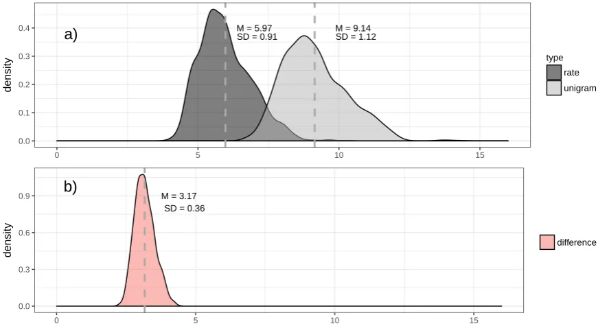
Figure5a) shows a density plot of the estimated entropic values across all texts and languages. Both unigram entropies and entropy rates show a unimodal distribution that is skewed to the right. The distribution of entropy differs clearly from the Gaussian – and therefore symmetric – distribution that is expected for the plug-in estimator under a two-fold null hypothesis: (1) that the true entropy is the same for all languages, and that (2) besides the bias in the entropy estimation, there is no additional bias constraining the distribution of entropy [61].

As we would expect, Figure 5 also shows that entropy rates are systematically lower than unigram entropies, since the former take co-text information into account, whereas the latter do not. To see this, remember that under stationarity, the entropy rate can be defined as a word entropy conditioned on a sufficiently large number of previous tokens (Equation 8), while the unigram entropy is not conditioned on the co-text. As conditioning reduces entropy [72], it is not surprising that entropy rates tend to fall below unigram entropies. Unigram entropies are distributed around a mean of 9.14 (SD = 1.12), whereas entropy rates have a lower mean of 5.97 (SD = 0.91). Figure5 shows that the difference between unigram entropies and entropy rates has a narrower distribution: it is distributed around a mean of ca. 3.17bits/wordwith a standard deviation of 0.36.

a)

M = 5.97SD = 0.91 M = 9.14SD = 1.12

0.0 0.1 0.2 0.3 0.4

0 5 10 15

density

type

rate

unigram

b)

M = 3.17 SD = 0.36

0.0 0.3 0.6 0.9

0 5 10 15

density

difference

Figure 5. The distribution of entropic measures in bits. a) Probability density of unigram entropies (light grey) and entropy rates (dark grey) across texts of the PBC (using 50Ktokens). MandSDare, respectively, the mean and the standard deviation of the values. A vertical dashed line indicates the meanM. b) The same for the difference between unigram entropies and entropy rates.

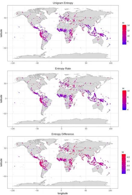
To further illustrate the diversity of entropies across languages of the world, Figure6 gives a map with unigram entropies, entropy rates and the difference between them for the PBC sample. The range of entropy values in bits per word is indicated by a colour scale from blue (low entropy) to red (high entropy). As can be seen in the upper map, there are high and low entropy areas across

(16)

16 of 34

Unigram Entropy

−180 −90 0 90 180

−50 0 50

latitude

8 10 12 14

H

Entropy Rate

−180 −90 0 90 180

−50 0 50

latitude

4 6 8 10

H

Entropy Difference

−180 −90 0 90 180

−50 0 50

longitude

latitude

2.5 3.0 3.5 4.0

H

Figure 6. World maps with unigram entropies (upper panel), entropy rates (middle panel), and the difference between them (lower panel), across texts of the PBC (using 50Ktokens), amounting to 1499 texts and 1115 languages.

(17)

17 of 34

the world. For example, languages in the Andean region of South America all have high unigram entropies (bright red). This is most likely due to their high morphological complexity, resulting in a wide range of word types, which were shown to correlate with word entropies [76]. Further areas of generally high entropies include Northern Eurasia, Eastern Africa, and North America. In contrast, Meso-America, Sub-Saharan Africa und South-East Asia are areas of relatively low word entropies (purple and blue). A similar pattern holds for entropy rates (middle panel), though they are generally lower. The difference between unigram entropies and entropy rates, on the other hand, is more narrowly distributed (as seen also in Figure5).

5.3. Correlation between unigram entropy and entropy rate

The density plot for unigram entropies in Figure5 looks like a slightly wider version of the entropy rate density plot – just shifted to the right of the scale. This suggests that unigram entropies and entropy rates might be correlated. Figure7 confirms this by plotting unigram entropies on the x-axis versus entropy rates on the y-axis for each given text. The linearity of the relationship tends to increase as text length increases (from 30K tokens onwards) as shown in Fig. 8. The fact that this holds for all entropy estimators is not surprising as they are strongly correlated (AppendixD).

In AppendixEwe also give correlations between unigram entropy values for all 9 estimation methods and entropy rates. The Pearson correlations are strong (between r = 0.95 andr = 0.99, withp<0.0001). This illustrates empirically that despite the conceptual difference between unigram entropies and entropy rates, there is a strong underlying connection between them. Namely, a linear model fitted through the points in Figure7(left panel) can be specified as

ˆ

h(T) =−1.12+0.78 ˆH1(T). (12)

Via Equation12we can convert unigram entropies into entropy rates with a variance of 0.035. More generally, word entropy rates ˆh(T)and unigram entropies ˆH1(T)are linked by a linear relationship:

ˆ

h(T) =k1+k2Hˆ1(T), (13)

wherek1andk2are constants.

The right panels of Figure7plot the same relationship between unigram entropies and entropy rates facetted by geographic macro areas taken from Glottolog 2.7 [77]. These macro areas are generally considered relevant from a linguistic typology point of view. It is apparent from this plot that the linear relationship extrapolates across these different areas of the world.

6. Discussion

6.1. Entropy estimation and stabilization

In Section5.1, we set out to establish stabilization points for both unigram entropies and entropy rates. We have illustrated that – independent of the estimation method – texts of 50K tokens are sufficient to estimate values with standard deviations below 0.1. This was shown across 21 languages of the EPC. Similar results are found for 32 languages of different language families in AppendixC. Furthermore, AppendixDillustrates that there are generally strong correlations between different entropy estimation methods – despite their differing stabilization properties. Finally, AppendixF gives Pearson correlations between unigram entropies of the PBC, EPC, and UDHR. These are also strong (around 0.8) – despite the differences in registers and styles as well as text sizes. Overall, our analyses converge to support the claim that entropy rankings of languages are stable at 50K tokens.

(18)

18 of 34

r = 0.95, p < 0.0001

4 5 6 7 8 9

8 10 12

Unigram Entropy (NSB)

Entrop

y Rate

North America Papunesia South America

Africa Australia Eurasia

8 10 12 8 10 12 8 10 12

4 5 6 7 8 9

Unigram Entropy (NSB)

Entrop

y Rate

Figure 7. Linear relationship between unigram entropies approximated with the NSB estimator (x-axis) and entropy rates (y-axis) for 1495 PBC texts (50K tokens) across 1112 languages. Four texts (Ancient Hebrew (hbo), Eastern Canadian Inuktitut (ike), Kalaallisut (kal), and Northwest Alaska Inupiatun (esk)) were excluded here, since they have extremely high values of more than 13 bits/word. In the left panel, a linear regression model is given as blue line, a local regression smoother is given as red dashed line. The Pearson correlation coefficient isr=0.95. In the right panels, plots are facetted by macro areas across the world. Macro areas are taken from Glottolog 2.7 [77]. Linear regression models are given as coloured lines with 95% confidence intervals.

CS NSB Shrink

Lap SG minimax

ML MM Jeff

0 25000 50000 75000 100000 0 25000 50000 75000 100000 0 25000 50000 75000 100000

0.7 0.8 0.9

Number of Tokens

P

earson Correlation betw

een Unigr

am Entrop

y and Entrop

y Rate

Figure 8. Pearson correlation between unigram entropy and entropy rate (y-axis) as a function of text length (x-axis). Each correlation is calculated over the 21 languages of the EPC corpus. All nine unigram entropy estimators are considered.

(19)

19 of 34

6.2. Entropy diversity across languages of the world

In Section5.2, we estimated word entropies for a sample of more than 1000 languages of the PBC. We find that unigram entropies cluster around a mean value of about 9 bits/word, while entropy rates fall closer to a mean of 6 bits/word. It is remarkable that given the wide range of potential entropies – from 0 to ca. 14 – most natural languages fall on a relatively narrow spectrum.8Unigram entropies mainly fall in the range between 7 to 12 bits/word, and entropy rates in the range between 4 to 9 bits/word. Thus, each only covers around 40% of the scale.

This suggests that there are pressures at play which keep word entropies in a relatively narrow range. We argue that these pressures are related to the trade-off between the learnability and

expressivity of communication systems. A (hypothetical) language with maximum word entropy would have a vast (potentially infinite) number of word forms of equal probability, and would be hard (or impossible) to learn. A language with minimum word entropy, on the other hand, would repeat the same word forms over and over again, and lack expressivity. Natural languages fall in a narrow range between these extremes. Kirbyet al.[78] illustrate how this trade-off effects the evolution of languages by using iterated learning experiments and computational simulations.

The trade-off is also obvious in optimization models of communication, which are based on two major principles:entropy minimizationandmaximization of mutual informationbetween meanings and word forms [40]. Entropy minimization is linked with learnability: fewer word forms are easier to learn (see [79] for other cognitive costs associated with entropy). Whereas mutual information maximization is linked with expressivity via the form/meaning mappings available in a communication system. Note that a fundamental property in information theoretic models of communication is thatMI, the mutual information between word forms and meanings, cannot exceed the entropy, i.e. [37]

MI ≤H (14)

The lower the entropy, the lower the potential for expressivity. This may shed light on the right-skeweness of the entropy distribution in Figure5. Displacing the distribution to the left or skewing it towards low values would compromise expressivity. In contrast, skewing it towards the right increases the potential for expressivity according to Eq.14, though this comes with a learnability cost.

Further support for pressure to increase entropy to warrant sufficient expressivity (Eq.14) comes from the fact that there is no language with less than 6 bits/word (unigram entropy) for neither the PBC nor the EPC. There is only one language in the UDHR that has a slightly lower unigram entropy – a Zapotecan language of Meso-America (zam). It has a fairly small corpus size (1067 tokens), and the same language has more than 8 bits/word in the PBC.

Despite the fact that natural languages do not populate the whole range of possible word entropies, there can still be remarkable differences. Some of the languages at the low-entropy end are Tok Pisin, Bislama (Creole languages), and Sango (Atlantic-Congo language of Western Africa). These have unigram entropies of around 6.7 bits/word. Languages to the high-end include Greenlandic Inuktitut and Ancient Hebrew – with entropies around 14 bits/word. Note that this is not to say that Greenlandic Inuktitut or Ancient Hebrew are “better” or “worse” communication systems than Creole languages or Sango. Such an assessment is misleading for two reasons: First, information encoding happens in different linguistic (and non-linguistic) dimensions, not just at the word level. We are only just starting to understand the interactions between these levels from an information-theoretic perspective [10]. Second, if we assume that natural languages are used for communication, then both learnability and expressivity are equally desirable features. Any

8 _{It is non-trivial to find an upper limit for the maximum word entropy of natural languages. In theory, word entropy could}

be infinite given that the range of word types is potentially infinite. However, in practice the highest entropy languages range only up to ca. 14bits/word.

(20)

20 of 34

combination of the two arises in the evolution of languages due to adaptive pressures. There is nothing “better” or “worse” about learnability or expressivityper se.

We are just beginning to understand the driving forces involved when languages develop extremely high or low word entropies. For example, Bentzet al.[12] as well as Bentz and Berdicevskis [18] argue that specific learning pressures reduce word entropy over time. As a consequence, different scenarios of language learning, transmission and contact might lead to global patterns of low and high entropy areas [14]. Developing and testing entropy estimation methods is the necessary foundation to further unravel the factors and causes of word entropy evolution and change.

6.3. Correlation between unigram entropies and entropy rates

Finally, in Section5.3, we found a strong correlation between unigram entropies and entropy rates. This is somewhat surprising, as we would expect that the co-text has a variable effect on the information content of words, and that this might differ across languages too. But what we actually find is that the co-text effect is (relatively) constant across languages. To put it differently, knowing the co-text of words decreases their uncertainty – or information content – by roughly the same amount, regardless of the language. Thus, entropy rates are systematically lower than unigram entropies – by 3.17 bits/word on average.

Notably, this result is in line with earlier findings by Montemurro and Zanette [8,9]. They have reported – for samples of 8 and 75 languages respectively – that the difference between word entropy rates for textswith randomized word orderand those of textwith original word orderis about 3.5 bits/word. Note that the word entropy rate given randomized word order is conceptually the same as unigram entropies, since any dependencies between words are destroyed via randomization [8] (technically all the tokens of the sequence become independent and identically distributed variables [72, p. 75]). Montemurro and Zanette [8,9] also show that while the average information content of words might differ across languages, the co-text reduces the information content of words by a constant amount. They interpret this as a universal property of languages. Also, we have shown that the entropy difference has a smaller variance than the original unigram entropies and entropy rates, again consistent with Montemurro and Zanette’s findings (Fig.5).

As a practical result, the entropy rate is a linear function of unigram entropy, and can be straightforwardly predicted from it. To our knowledge, we have provided the first empirical evidence for a linear dependency between the entropy rate and unigram entropy (Fig.7). Interestingly, we have shown that this linearity of the relationship increases as text length increases (Fig.8). A mathematical investigation of the origins of this linear relationship should be the subject of future research.

Note that estimating entropy rates requires searching strings of lengthi−1, whereiis the index running through all tokens of a text. Asiincreases, the CPU time per additional word token increases linearly. In contrast, unigram entropies can be estimated based on dictionaries of word types and their token frequencies, and the processing time per additional word token is constant. Hence, Equation12 can help to reduce processing costs considerably.

7. Conclusions

The entropy, average information content, uncertainty or choice associated with words is a core information-theoretic property of natural languages. Understanding the diversity of word entropies requires an interdisciplinary discourse between information theory, quantitative linguistics, computational linguistics, psycholinguistics, language typology, as well as historical and evolutionary linguistics.

As a first step, we have here established word entropy stabilization points for 21 languages using the European Parliament Corpus. We illustrated that word entropies can be reliably estimated with text sizes of > 50K. Based on these findings, we estimated entropies across 1499 texts and 1115 languages of the Parallel Bible Corpus. These analyses shed light on both the diversity of languages, and the underlying universal pressures that shape them. While the information encoding

(21)

21 of 34

strategies of individual languages might vary considerably across the world, they all need to adhere to fundamental principles of information transfer. In this context,learnabilityandexpressivityseem to emerge as fundamental constraints on language variation.

Furthermore, we have shown that there is a strong linear relationship between block entropies and entropy rates, which holds across different macro areas of the world’s languages. The theoretical implication of this finding is that co-text effects on the information content of words are relatively similar regardless of the language we are looking at. The practical implication is that entropy rates can be approximated by using unigram entropies, thus reducing processing costs.

Acknowledgments: We are grateful to Ł. D˛ebowski for helpful discussions. CB was funded by the German Research Foundation (DFG FOR 2237: Project “Words, Bones, Genes, Tools: Tracking Linguistic, Cultural, and Biological Trajectories of the Human Past”), and by the ERC Advanced Grant 324246 EVOLAEMP. RFC was funded by the grants 2014SGR 890 (MACDA) from AGAUR (Generalitat de Catalunya) and also the APCOM project (TIN2014-57226-P) from MINECO (Ministerio de Economia y Competitividad).

Author Contributions: CB, DA and RFC conceived and designed the experiments; CB and DA performed the experiments; CB and DA analyzed the data; MC contributed materials; CB and RFC wrote the paper.

Conflicts of Interest:The authors declare no conflict of interest.

Abbreviations

The following abbreviations are used in this manuscript:

EPC: European Parliament Corpus PBC: Parallel Bible Corpus

UDHR: Universal Declaration of Human Rights NSB: Nemenman-Shafee-Bialek

Appendix A Text pre-processing

Appendix A.1 Converting letters to lower case

This is done via the functiontolower()in R. Cross-linguistically, it is common that upper case letters are used to indicate the beginning of a sentence, i.e.theandThe. In this case, we are not dealing with different word types from a grammatical or semantic perspective, but with two alternative writings of the same word type. Therefore, it is common practice to convert all letters to lower case as a pre-processing step.

Note that – in a few cases – conversion of letters to lower case can create polysemy. Namely, when upper and lower case actually distinguish separate word types. For example, in German, verbs can be nominalized by using an upper case initial letter:fahren‘drive’, anddas Fahren‘the driving’ are two different word types. This difference is neutralized when all letters are set to lower case.

Appendix A.2 Removal of punctuation

All three corpora (EPC, PBC, UDHR) are encoded in unicode UTF-8, which generally makes them accessible to the same automated processing tools. However, there are subtle difference with regards to orthographic practices. While the EPC follows common orthographic conventions, the PBC and UDHR are specifically curated to delimit word types and punctuation byadditional white spaces. Take the following example sentences:

Although, as you will have seen, the dreaded ’millennium bug’ failed to materialise,[...]

EPC (English, line 3)

And God said , let there be light . And there was light .[...]

(22)

22 of 34

PBC (English, Genesis 1:3)

Furthermore , no distinction shall be made on the basis of the political , jurisdictional or international status of the country[...]

UDHR (English, paragraph 3)

The automatically added – and manually checked – white spaces in the PBC and UDHR make cross-linguistic analyses of word types more reliable. This is especially helpful since we deal with hundreds of languages, representing different writing systems and scripts. For instance, characters like apostrophes and hyphens are often ambiguous as to whether they are part of a word type, or being used as punctuation.

Apostrophes can indicate contractions as in English she’s representing she is. Here, the apostrophe functions as a punctuation mark. In other cases, however, it might reflect phonetic distinctions. For instance, glottal stops or ejectives as in the Mayan language K’iche’ (quc). Take the wordq’atb’altzijmeaning ‘everyone’. Here, the apostrophes are part of the word type, and should not be removed. To disambiguate these different usages the PBC and UDHR would giveshe ’ sversus

q’atb’altzij.

Another example are raised numbers indicating tone distinctions. In the Usila Chinantec (cuc) version of the Bible, for instance, the proper nameAbrahamis rendered asA3brang23. These numbers indicate differences in pitch when pronouncing certain word types, and are hence part of their lexical (and grammatical) properties. If tone numbers are interpreted instead as non-alphanumeric indications of footnotes, then words might be erroneously split into separate parts, e.g. A brang. Again, the PBC and UDHR use white spaces to disambiguate here.

Given this difference in the usage of white spaces, we use two different strategies to remove punctuation:

1. For the EPC, we use the regular expression ‘\\W+’ in combination with the R functionstrsplit()

to split strings of UTF-8 characters on punctuation and white spaces.

2. For the PBC and UDHR, we define a regular expression meaning “at least one alpha-numeric UTF-8 character between white spaces” which would be written as:

.*[[:alpha:]].*

This regex can then be matched with the respective text to yield word types. This is done via the functionsregexpr()andregmatches()in R.

Appendix B Advanced entropy estimators

As outlined in Section3.2, to estimate the entropy given in Equation3reliably, the critical part is to get a good approximation of the probability of words. Hence, p(wi) is the critical variable to

be approximated with highest possible precision. Henceforth, estimated probabilities are denoted as ˆ

p(wi), and estimated entropies correspondingly ˆH.

Using frequency counts from a subsample, i.e. using

ˆ

p(wi)ML= fi

∑V j=1fj

, (15)

is generally referred to as themaximum likelihood (ML) method. Note that the denominator here is equivalent to the total number of tokens, denoted asNin the following. Plugging15into3yields the estimated entropy as [59]

ˆ

HML=−

V

∑

i=1 ˆ

p(wi)ML log2(pˆ(wi)ML). (16)

(23)

23 of 34

The ML method yields reliable results for situations whereNV, i.e. the number of tokens is much bigger than the number of types [59, p. 1470]. In other words, it is reliable for a small ratio of word types to word tokensV/N. Since in natural language this ratio is typically big for small texts, and only decreases withN[66,80], entropy estimation tends to be unreliable for small texts. However, since Shannon’s original proposal in the 1950s a range of entropy estimators have been proposed to overcome the underestimation bias [see59, for an overview]. Some of these are discussed in turn.

Appendix B.1 The Miller-Madow estimator

For example, theMiller-Madow(MM) estimator [59, p. 1471] tries to reduce the bias by adding a correction to the ML estimated entropy such that

ˆ

HMM =HˆML+ M>0−1

2N , (17)

whereM>0refers to the number of types with token frequencies > 0, i.e. V in our definition. Note that the correction V−1

2N is relatively big for theN <Vscenario, and relatively small for theN> V

scenario. Hence, it counterbalances the underestimation bias in the N < V scenario of small text sizes.

Appendix B.2 Bayesian estimators

Another set of estimators derives from estimatingp(wi)within a Bayesian framework using the

Dirichlet distribution witha1,a2, ...,aVas priors such that

ˆ

p(wi)Bayes= fi

+ai

N+A, (18)

where ai values essentially “flatten out” the distribution of frequency counts to overcome the bias

towards short tailed distributions (with small V). Besides N, we have A = _∑V_i₌₁ai added to the

denominator [81, p. 302-303].

Now, depending on which priors exactly we choose, we end up with different estimated entropies (see also Table 1 in Hausser and Strimmer [59, p. 1471]). A uniformJeffreys priorofai=1/2

gives us ˆHJe f f, a uniformLaplace priorofai =1 gives us ˆHLap, a uniformPerks priorofai=1/Vgives

us ˆHSG, after Schürmann & Grassberger [6], who proposed to use this prior. Finally, the so-called minimax prior ofai=

√

N/Vyields ˆHminimax.

Furthermore, the most recent – and arguably least biased – entropy estimator based on a Bayesian framework is the Nemenman-Shafee-Bialek (NSB) estimator [52]. Nemenman et al.[52, p. 5] illustrate that the entropies estimated with the other priors proposed above will be strongly influenced by the prior distributions and only recover after a relatively big number of tokens has been sampled. Instead of directly using any specific Dirichlet prior, they form priors as weighted sums of the different Dirichlet priors, which they callinfinite Dirichlet mixture priors. The resulting entropy estimates ˆHNSB_{turn out to be robust across the whole range of sample sizes.}

Appendix B.3 The Chao-Shen estimator

Chao and Shen [82, p. 432] propose to overcome the problem of overestimating the probability of each type (in their case species instead of word types) by first estimating the so-called sample coverage as

ˆ

C=1−m1

N, (19)

wherem1is the number of types with frequency 1 in the sample (i.e. hapax legomena). The idea is that the number of types not represented by tokens is roughly the same as the number of types with

(24)

24 of 34

frequency 1. In this case, the sample coverage reflects the conditional probability of getting a new type if a token is added to the sampleN. This probability is then multiplied with the simple ML estimate ˆp(wi)MLto get the so-calledGood-Turingestimated probability of a type

ˆ

p(wi)GT=

1− m1

N

ˆ

p(wi)ML. (20)

Furthermore, Chao and Shen [82, p. 431] suggest to use theHorvitz-Thompson estimatorto modify the estimated entropy ˆHML. This estimator is based on the rationale that if N tokens have been sampled with replacement, then the probability of theith type not being represented by a specific token is 1−pˆ(wi)GT. Thus, the probability of the ith type not being represented by any token is

(1−pˆ(wi)GT)N, and, inversely, the probability of appearing at least once in a sample of N tokens

is 1−(1−p(wi)GT)N. The full specification of the Horvitz-Thompson estimator, with Good-Turing

probability estimates, is then

ˆ

HCS =−

V

∑

i=1 ˆ

p(wi)GTlog2(pˆ(wi)GT)

1−(1−pˆ(wi)GT)N

. (21)

Appendix B.4 The James-Stein shrinkage estimator

Finally, Hausser and Strimmer [59, p. 1472] put forward an entropy estimator based on the so-calledJames-Stein shrinkage. According to this approach the estimated probability per type is

ˆ

p(wi)shrink=λpˆ(wi)target+ (1−λ)pˆ(wi)ML, (22)

whereλ∈[0, 1]is the shrinkage intensity and ˆp(wi)targetis the so-called “shrinkage target”. Hausser

and Strimmer [59, p. 1473] suggest to use the maximum entropy distribution as a target, i.e.pˆ(wi)target= 1

V. This yields

ˆ

p(wi)shrink=

λ

V + (1−λ)pˆ(wi)

ML_. ₍₂₃₎

The idea here is that the estimated probability ˆp(wi)shrinkconsists of two additive components,

λ V and

(1−λ)pˆ(wi)MLrespectively. In the full shrinkage case (λ=1) Equation23yields

ˆ

p(wi)shrink=

1

V, (24)

i.e. uniform probabilities that will yield maximum entropy. In the lowest shrinkage case (λ = 0)

Equation23yields

ˆ

p(wi)shrink=pˆ(wi)ML, (25)

i.e. the ML estimation that is biased towards low entropy. Given empirical data, the true probability is very likely to lie somewhere in between these two cases and hence 0<λ<1. In fact, Hausser and

Strimmer [59, p. 1481] show that the optimal shrinkageλ* can be calculated analytically and without

knowing the true probabilities p(wi). Given the optimal shrinkage, the probability ˆp(wi)shrinkcan

then be plugged into the original entropy equation to yield

(25)

25 of 34

ˆ

Hshrink=−

V

∑

i=1 ˆ

p(wi)shrinklog2pˆ(wi)shrink. (26)

Overall, 9 different entropy estimators were outlined here, from the most simple and “naive” maximum likelihood estimator to very advanced and arguably much less biased estimators such as the NSB estimator. All of these are available for estimation via theRpackageentropy[75].

Appendix C Stabilization of entropy rates for 32 languages of the Parallel Bible Corpus

Here we report entropy rate stabilization results for 32 languages of the PBC (Figure9and10). These 32 languages were chosen to represent the major language families across the world. They give a better overview of the linguistic diversity than the 21 mainly Indo-European languages represented in the EPC. The methodology is the same as for the original analyses with the 21 EPC languages described in the main paper.

(26)

26 of 34 Tok Pisin Creole Totonac Totonacan Turkish Turkic

Tzotzil (Venustiano Carranza) Mayan Vietnamese Austroasiatic Warlpiri Pama−Nyungan Yagua Peba−Yagua Zapotec (Isthmus) Otomanguean Mufian Torricelli Nahuatl Uto−Aztecan Quechua (Cusco) Quechuan Saami (Northern) Uralic Secoya Tucanoan Severn Ojibwa Algic Shipibo−Conibo Pano−Tacanan Thai Tai−Kadai Fore

Nuclear Trans New Guinea

Garifuna Arawakan Guarani (Paraguayan) Tupian Hakka Chinese Sino−Tibetan Hausa Afro−Asiatic Indonesian Austronesian Kannada Dravidian Korean Isolate Alamblak Sepik Arabela Zaparoan Carib Cariban Chechen Nakh−Daghestanian Cherokee Iroquoian Dinka (SW) Nilotic Efik Atlantic−Congo English Indo−European

0 25000 50000 75000 100000 0 25000 50000 75000 100000 0 25000 50000 75000 100000 0 25000 50000 75000 100000 0 25000 50000 75000 100000 0 25000 50000 75000 100000 0 25000 50000 75000 100000 0 25000 50000 75000 100000

4 5 6 7 8 4 5 6 7 8 4 5 6 7 8 4 5 6 7 8

Estimated Entrop

y (bits/w

ord)

Figure 9. Entropy rates as a function of text length across 32 languages of the PBC. Languages were chosen to represent some of the major language families across the world. Entropy rates are estimated on prefixes of the text sequence increasing by 1K tokens as in Fig.1. Hence there are 100 points along the x-axis. The language names and families are taken from Glottolog 2.7 [77] and given above the plots.

Preprints

doi:10.20944/preprints201704.0180.v1

Entropy

2017

,

19

, , 275;