Morphology
Wei Lu 1,2,*, Mengjie Zeng1,2, Ling Wang1,2, Hui Luo1,2, and Yiming Deng3 1 College of Engineering, Nanjing Agricultural University, Nanjing 210031, China
2 Key Laboratory of Intelligent Agricultural Equipment in Jiangsu Province, Nanjing Agricultural University, Nanjing 210031, China
3 NDE Laboratory, College of Engineering, Michigan State University, East Lansing 48824, USA * Correspondence: [email protected]
Abstract: An improved anti-noise morphology vision navigation algorithm is proposed for intelligent tractor tillage in a complex agricultural field environment. Firstly, the two key steps, Guided Filtering and improved anti-noise morphology navigation line extraction, were addressed in detail. Then the experiments were carried out in order to verify the effectiveness and advancement of the presented algorithm. Finally, the optimal template and its application condition were studied for improving the image processing speed. The comparison experiment results show that the YCbCr color space has minimum time consumption, 0.094 s, compared with HSV, HIS and 2R-G-B color spaces. The Guided Filtering method can enhance the new & old soil boundary effectively than any other methods such as Tarel, Multi-scale Retinex, Wavelet-based Retinex and Homomorphic Filtering, meanwhile, has the fastest processing speed of 0.113 s. The extracted soil boundary line of the improved anti-noise morphology algorithm has best precision and speed compared with other operators such as Sobel, Roberts, Prewitt and Log. After comparing different size of image template, the optimal template with the size of 140×260 pixels can meet high precision vision navigation while the course deviation angle is not more than 7.5°. The maximum tractor speed of the optimal template and global template are 51.41 km/h and 27.47 km/h respectively which can meet real-time vision navigation requirement of the smart tractor tillage operation in the field. The experimental vision navigation results demonstrated the feasibility of the autonomous vision navigation for tractor tillage operation in the field using the new & old soil boundary line extracted by the proposed improved anti-noise morphology algorithm which has broad application prospect.
Keywords: intelligent tractor; vision navigation; improved anti-noise morphology; boundary line; Guided Filtering
1. Introduction
Agricultural machinery [1] automatic navigation system is a key part of the smart tractor [2] for implementing precision agriculture which can free drivers from the boring work as well as improve the work quality. Global positioning technique by using GPS or GNSS [3-5] is applied to automatic navigation of unmanned tractors during tillage operation in the field to obtain absolute geographic coordinates dynamically, whereas the navigation precision is heavily influenced by the inclination angle of the field surface, meteorological condition and the strength of satellite navigation signal especially in remote areas. Inertial sensors [6,7] which have a large error in long-distance navigation can only be used as compensation for short-range position correction. Therefore, vision navigation [8] as a popular method in autonomous vehicles, mobile robot, and aircraft has been introduced to intelligent agricultural machinery. The Silsoe Research Institute of the United Kingdom focused on machine vision-based automatic navigation technology and established an extended Kalman filter model for field vehicles. The research team in Cemagref University in France proposed the MRF
algorithm to deal with the edge recognition problem of harvested crops to identify crop rows from a multi-feature perspective. Nishiwaki Kentaro of Japan used a pattern matching method according to the character of the distribution shape between rice rows to measure vehicle position. Carnegie Mellon University combined a visual odometry system with an aided inertial navigation filter to produce a robust tractor navigation system with the accuracy in meters on the rural and urban roads that does not rely on external infrastructure. Aiming at crop harvest and management operation, China Agricultural University, Nanjing Agricultural University, and Nanjing Forestry University have proposed plant navigation line extraction algorithms such as filtering method based on image scanning, wavelet transform, and optimized Hough transform respectively to improve recognition of plant navigation line.
A local autonomous navigation method by applying the boundary line of new & old soil was presented in this paper while the tractor works in tillage mode inspired by the existed plant line navigation method. Moreover, the fast image processing algorithm using optimized templates combined with Guided Filtering [9-12], improved anti-noise morphology, and Hough transformation [13,14] was proposed to meet the practical application of agricultural tillage.
2. Materials and Methods
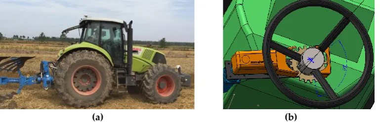
The intelligent tractor updated from a traditional tractor with the type of AXION 850(CLAAS) by adding a tractor driving robot as shown in Figure 1. The tractor driving robot consists of a steering arm, a gears-shifting arm, a break leg, a clutch leg and an accelerator leg which can operate a tractor imitating a tractor driver. Moreover, a camera (BLUELOVER, resolution 1280×980) and an RTK GPS (X10, Huace Co., China) were installed on the tractor for automated guided operation.
The tillage procedure of the intelligent tractor includes two steps. Firstly, the tractor tills a round line under manual control or teleoperation control to create a boundary of new & old soil. Then the tractor works at autonomous navigation model based on the boundary calculated by using Guided Filtering, improved anti-noise morphology and Hough transformation in sequence in consideration of the severe randomness and ununiform of agricultural filed environment.
(a) (b)
Figure 1. Intelligent tractor platform. (a) Tractor platform; (b) Steering configuration.
3. Guided Filtering
3.1. Local linear model
The local linear model is mostly used for non-analytic functions which is defined as the adjacent points on a function have a linear relationship with others. The definition shows that a complex function can be represented by multiple adjacent local simple linear functions. Each point value can be obtained by averaging the weights of all the linear functions which including the point.
Denote the input image as 𝐼 which is the image to be filtered, and the output as 𝑞. The local
linear model of guided filter assumes that 𝑞 is a linear transform of the 𝐼 in a window 𝑤𝑘 centered
at pixel 𝑘, so 𝑞𝑖 which is a pixel in 𝑞 can be expressed as
𝑞𝑖= 𝑎𝑘𝐼𝑖+ 𝑏𝑘 , ∀𝑖 ∈ 𝑤𝑘 (1)
Where 𝑎 and 𝑏 are the coefficients of the linear function when the window center is located at
3.2 Local linear model solution
The process of calculating linear function coefficients is called linear regression. Define the true
value of the fitting function p, so the difference value between 𝑝 and the actual output is as below.
𝐸(𝑎𝑘, 𝑏𝑘) = ∑𝑖∈𝑤𝑘((𝑎𝑘𝐼𝑖+ 𝑏𝑘− 𝑝𝑖)2+ 𝜀𝑎𝑘2) (3)
Where 𝑝 denotes the image to be filtered; 𝜀 is a parameter used for adjusting filtering effect
whose purpose is to prevent the amount of a value from being too large. The filtering effect improves
remarkably with the increasement of 𝜀. Minimizing formula (3) to defines a least square problem
within a window 𝑤𝑘, its solution is given by:
𝑎𝑘= 1
|𝑤|∑𝑖∈𝑤𝑘𝐼𝑖𝑝𝑖−𝜇𝑘𝑝𝑘
𝜎𝑘2+𝜀 (4)
𝑏𝑘= 𝑝𝑘− 𝑎𝑘𝜇𝑘 (5)
In which 𝜎𝑘2 and 𝜇𝑘 are the variance and mean of 𝐼 in 𝑤𝑘, 𝑝𝑘 is the average value of the
image 𝑝 to be filtered in the window, |𝑤| denotes the number of pixels contained in the window.
In view of the fact that a pixel can be described by multiple linear functions, all linear function values containing the point are weighted averaged when calculating the output value of the point in the formula below.
𝑞𝑖 = 1
|𝑤|∑𝑖∈𝑤𝑘(𝑎𝑘𝐼𝑖+ 𝑏𝑘)= 𝑎𝜏𝐼𝑖+ 𝑏𝜏 (6)
The process of weighted averaging is a linear translational variation filtering process, and the calculation of the Guided Filtering is based on this process.
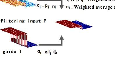
The processing process of the guided filter is shown in Figure 2. Among them, the definition of
a guiding graph is 𝑃, and the relationship between 𝑃 and the original graph 𝐼 is represented by a
local linear model definition. In the figure, 𝑞 is the linear transformation of the original image 𝐼 in
the window adjacent to a pixel value, and 𝑎 and 𝑏 are the coefficients of the linear function of the
window center at the pixel value. The output pixel value 𝑞 is linearly multiplied by the input image
𝐼, so 𝑞 has a similar gradient to 𝐼. The edge characteristics of the original image 𝐼 are still preserved
in the image 𝑞 after being processed by the Guided Filtering process.
Figure 2. The Guided Filtering process.
4. Improved anti-noise morphology algorithm for image navigation line extraction
Introducing the concept of mathematical morphology [15-19] to the image edge detection operator can overcome the shortcomings of the classical operator [20-22], and greatly reduce the calculation amount. The paper proposed an improved anti-noise morphology algorithm for image navigation line extraction which selects a pair of smaller-scale structural elements for further anti-noise processing to extract image navigation line based on the edge feature.
coherent, and obtain more accurate edge localization. Whereas large-scale structural elements can reflect the large edge contours in the image and have good noise suppression effect. Therefore, small-scale structural elements were selected for obtaining complete edges in this paper.
The edge of the image is calculated as below:
𝑦𝑑 = (((𝑓 ∘ 𝐴1) ⋅ 𝐴2) ⊕ 𝐴2) ∘ 𝐴2− (𝑓 ∘ 𝐴1) ⋅ 𝐴2 (7)
𝑦𝑒= (𝑓 ∘ 𝐴1) ⋅ 𝐴2− (((𝑓 ∘ 𝐴1) ⋅ 𝐴2)𝛩𝐴2) ⋅ 𝐴2 (8)
Where 𝐴1and 𝐴2 are two different structural elements:
𝐴1= [0,1,0; 1,1,1; 0,1,0]
𝐴2= [1,0,0; 1,0,0; 1,0,0];
𝑓 is the image after Guided Filtering treatment. The anti-noise morphology edge detection
operator is given as follows:
𝑦𝑑𝑒 = 𝑦𝑑+ 𝑦𝑒 (9) The edge image detected by equations (7) and (8) can obtain the edge details after the minimum
operation. For detecting more detailed edges as well as improving the anti-noise ability of 𝑦𝑑𝑒 under
the condition of equal noise, the noise immunity is defined as
𝑦 = 𝑦𝑑𝑒+ 𝐸𝑚𝑖𝑛 (10)
Where 𝐸𝑚𝑖𝑛 is 𝑚𝑖𝑛{ 𝑦𝑑, 𝑦𝑒}; 𝑦𝑑 is the edge detected by equation (7); 𝑦𝑒 is the edge detected by
equation (8); 𝑦𝑑𝑒 is the edge detected by equation (9).
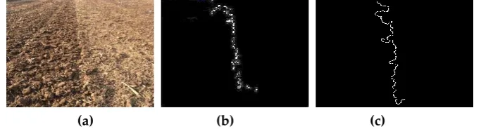
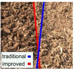
The new & old soil boundary line extracted by using the algorithm mentioned above is shown in Figure 3(c) compared with that extracted by color space conversion followed with threshold processing shown in Figure 3(b). There are remarkable errors at both ends of the navigation line in Figure 3(b) because of the calculation error caused by the truncation of the image. Whereas, it is obvious that the truncation error in Figure 3(c) is significantly improved for navigation line extraction.
(a) (b) (c)
Figure 3. The edge dealing. (a) Original; (b) Edge information; (c) Processed edge information.
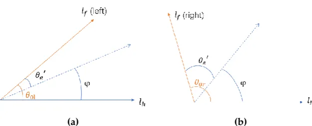
The tractor completed the first returning tillage manually, by human driving or tele-operational driving, before autonomous image aided navigation operation. The navigation line of the tractor is calculated by using Hough transformation from the processed new & old soil boundary in Figure 3. In the actual operation, the navigation line is attached to one side of the tractor. It is influenced by the angle of view of the camera position which results in an angular deviation between the calculated navigation line and the actual line. For this problem, the transverse line of the tractor is defined as
the horizontal line 𝑙ℎ. The forward direction line of the tractor is deviated in the camera image as
shown in Figure 4 where the front lines 𝑙𝑓 in the left view and right view are rotated to an acute
(a) (b)
Figure 4. Direction correction diagram. (a) Left view; (b) Right view.
For simplifying the adjustment algorithm of the navigation line, the actual direction angle 𝜃 of
the tractor is calculated as:
𝜃 = 𝜑 ⋅ 𝑘 (𝑘 =90°𝜃
0) (11)
Where 𝜑 denotes the navigation angle between the new & old soil boundary and the horizontal
line of the tractor extracted from the image. 𝜃0 is the angle between the front line and the horizontal
line in the image and equal to 𝜃0𝑙 and 𝜃0𝑟 respectively when the boundary line locates at the left
side and right side of the tractor.
During tractor navigation using new & old soil boundary line, 𝜃0 and 𝑘 are calculated as
initialization. Then the navigation angle 𝜃 is obtained after navigation line extraction from the
image.
The tractor needs to turn left if the navigation angle 𝜃 is not more than 90 degree otherwise it
need to turn right whether the boundary line locates at the left or right side of the tractor. The steering adjustment algorithm flowchart is a detailed algorithm flowchart of steering adjustment is shown in Figure 5.
Figure 5. Steering adjustment algorithm flowchart.
The detailed algorithm of improved anti-noise morphology is shown in Figure 6.
1. Convert grayscale image 𝑞 into binary image ℎ;
2. Narrow down the research template and select the area of interest 𝑓 in ℎ for research;
3. Select structural elements:
𝐴1= [0,1,0; 1,1,1; 0,1,0]
𝐴2= [1,0,0; 1,0,0; 1,0,0];
Figure 6. Improved anti-noise morphological algorithm.
5. Experiment
In this paper, the computer employed for the new & old soil boundary navigation line extraction is configured as follows: 64-bit Windows 10 operating system, 8G memory, and a 2-core processor Intel(R) Core(TM) i5-4200H CPU @ 2.80 GHz. The first experiment was carried out to verify the effectiveness of the proposed algorithm mentioned above using several tillage images of different farms. Secondly, the navigation algorithm was used for smart tractor tillage in an experimental farm of Nanjing Agricultural University, moreover, the optimal template was studied to improve the efficiency of the algorithm.
5.1. Effectiveness verification of the algorithm
5.1.1 Color space selection
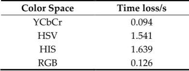
The time consumption and each optimal effect component of the YCbCr, HSV, HIS, and 2R-G-B [23-26] format images converted from the original image are shown in Table 1 and Figure 7, which indicate that the new & old soil boundary in the Cr component in YCbCr format image is clearest among all the gradation component images as well as fastest conversion speed, only 0.094s. Besides, the histogram of the best gradation component in each image, shown in Figure 8, denotes that the frequencies of I and V gradation components are constant to be zero, 2R-G-B gradation component has less obvious threshold segmentation pixel number, Cr gradation component has apparent threshold segmentation point at 15 pixels. So, the Cr component is selected for the identification of new & old soil boundary.
Table 1. Consumption contrast of different color spaces.
Color Space Time loss/s
YCbCr 0.094
HSV 1.541
HIS 1.639
RGB 0.126
𝑦𝑑= (((𝑓 ∘ 𝐴1) ⋅ 𝐴2) ⊕ 𝐴2) ∘ 𝐴2− (𝑓 ∘ 𝐴1) ⋅ 𝐴2
𝑦𝑒= (𝑓 ∘ 𝐴1) ⋅ 𝐴2− (((𝑓 ∘ 𝐴1) ⋅ 𝐴2)𝛩𝐴2) ⋅ 𝐴2;
5. Perform the minimum operation on the image edge obtained in step 4 to get the detail
edge:
𝐸𝑚𝑖𝑛= 𝑚𝑖𝑛{𝑦𝑑, 𝑦𝑒};
6. Edge extraction: 𝑦𝑑𝑒 = 𝑦𝑑+ 𝑦𝑒;
7. Sum the edges of the images in step 5 and step 6 to get the final image edge:
𝑦 = 𝑦𝑑𝑒+ 𝐸𝑚𝑖𝑛;
8. Filter and remove boundary objects in 𝑛;
9. Identify the new & old soil boundary lines and pseudo-color processing to determine the
(a) (b) (c) (d) (e)
Figure 7. Component graph of each other space. (a) Original; (b) Cr; (c) V; (d) I; (e) 2R-G-B.
Figure 8. Histogram comparison of Y, V, I, 2R-G-B.
5.1.2 Filtering method selection
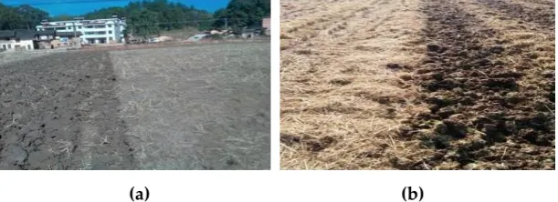
For improving the robustness of the algorithm, the images captured in weak and strong light environment, shown in Figure 9, were used for filtering methods selection because the illumination strength in the field is changeable and uncertain.
(a) (b)
Figure 9. Fields with different illumination strength. (a) Weak light intensity; (b) Strong light intensity.
(a) (b) (c)
(d) (e) (f)
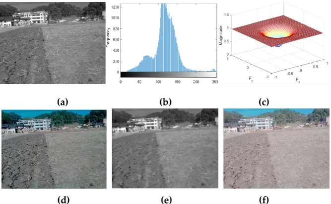
Figure 10. The process of the weak light intensity image using Homomorphic Filtering algorithm. (a) Grayscale; (b) Grayscale histogram; (c) Frequency response of the high pass filter; (d) Butterworth high pass Filtering; (e) Median Filtering; (f) Homomorphic Filtering.
(a) (b) (c)
(d) (e) (f)
Figure 11. The process of the strong light intensity image using Homomorphic Filtering algorithm. (a) Grayscale; (b) Grayscale histogram; (c) Frequency response of the high pass filter; (d) Butterworth high pass Filtering; (e) Median Filtering; (f) Homomorphic Filtering.
(a) (b) (c)
(d) (e) (f)
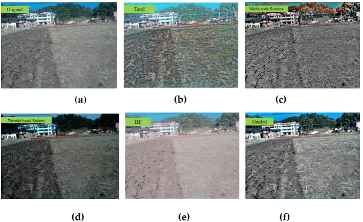
Figure 12. The input image and experiment results of the filtering algorithm. (a) Original; (b) Tarel; (c) Multi-scale Retinex; (d) Wavelet-based Retinex; (e) HF; (f) Guided.
The contrastive calculation time of the filtering algorithms mentioned above is shown in Table 2. Among them, the image processing time of the Guided Filtering algorithm is only 0.113 second. Followed by Multi-scale Retinex, HF, Tarel and Wavelet-based Retinex algorithms which take 0.552,0.867, 0.902 and 1.008 second respectively.
Table 2. The testing data to the different filtering methods.
Filtering method Highlighting Time loss/s
Tarel - 0.902
Multi-scale Retinex + 0.552
Wavelet-based Retinex + 1.008
HF - 0.867
Guided + 0.113
So, the Guided Filtering algorithm is selected for new & old soil boundary identification considered the image processing speed and the contrast of the new & old soil.
5.1.3 Navigation line extraction using improved anti-noise morphology algorithm
The edge extraction results and the Hough transform results of the image by using traditional morphology and improved anti-noise morphology algorithms are shown in Figure 13 and Figure 14, respectively. The improved anti-noise morphology algorithm can eliminate the soil boundary noise made by the traditional morphology algorithm because of the adopted double structure and minimum operation. The navigation error can decrease from 10° by using the traditional morphology algorithm to 0.5° by using the improved anti-noise morphology.
(a) (b)
Figure 14. Results of Hough transform.
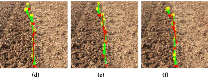
The comparison edge extraction result between the improved anti-noise morphology algorithm and the popular edge extraction algorithms such as Sobel [36-40], Roberts [41,42], Prewitt [43,44] and Log [45] is shown in Figure 15. There are some breakages in the extracted edges by using the later four algorithms which will lead to large error during navigation line identification processing. Moreover, the longest extracted navigation line created by using the improved anti-noise morphology combined with Hough transform method has best precision compared with others, in Figure 16.
(a) (b) (c)
(d) (e) (f)
Figure 15. The results of edge detection. (a) Original; (b) Sobel; (c) Roberts; (d) Prewitt; (e) Log; (f) Advanced morphology.
(d) (e) (f)
Figure 16. The longest line of operators. (a) Original; (b) Sobel; (c) Roberts; (d) Prewitt; (e) Log; (f) Advanced morphology.
The time consumption of the above algorithms is shown in Table 3. Among them, the time consumption of the improved anti-noise morphology is minimal, followed by the Sobel operator, the Roberts operator, the Prewitt operator, and the Log operator. The longest line is used as the tractor navigation line to calculate the orientation error for tractor steering adjustment.
Table 3. Time consumption contrast of different edge operators.
Edge operators Time loss/s Sobel
Roberts Prewitt
Log
advanced morphology
0.089 0.090 0.090 0.096 0.073
5.1.4 Image template optimization
In order to further improve the real-time vision navigation during tractor linear tillage operation, the appropriate image should be cropped from the whole original image because a larger size picture needs more computer processing time. Tractor tillage operation includes two work mode, i.e. linear mode and turning mode. During the linear mode, the longest line of new & old soil boundary is created using the above-advanced morphology algorithm firstly. Then a rectangle centered at the middle of the longest line is used to crop a part of the original picture for tractor navigation line calculation because the position and the navigation angle of the soil boundary line change a little. During the turning mode, the original image should be adopted for tractor navigation because the position of the soil boundary in the image varies a lot which leads to the boundary information loss in the rectangle.
The optimization template selection scheme is as follows:
(1) The original image is grayscale transformed and uniformly scaled to 816×612 pixels.
(2) The middle of the longest line is used as a reference point.
(3) Different size rectangles centered at the reference point are used for navigation precision
(a) (b)
Figure 17. Different templates. (a) Rectangular frame selection; (b) Navigation line extraction result.
The experimental results, shown in Figure 17(b), denote that the navigation angle error decreases significantly when the length and width are not less than 260 and 140 pixels respectively. Because the boundary information decreases with the template size shrinking. when the size of the image boundary signal is not more than that of the background noise when the image size of the template is less than 140×260 pixels. And the algorithm processing costs only 47 ms for the template with the size of 140×260 pixels compared with that of the template with 816×612 pixels which time consumption is 520 ms.
5.2 Navigation experiment in the field
The vision autonomous navigation experiment using the proposed new & old soil boundary was carried out in the farmland of Nanjing Agricultural University using a tractor (CLAAS AXION 850 model) equipped with the tractor driving robot developed by our team. For comparing the navigation precision, an RTK GPS (X10, Huace Co., China) was applied and the navigation line was used as the reference, as shown in Figure 18.
Figure 18. Tractor experiment diagram.
Figure 19. Navigation line extraction.
Firstly, the applied condition of the optimal template of 140×260 pixels was studied by changing
the deviation angle 𝜃e between the tractor longitudinal direction and the new & old soil boundary
line. The experimental results indicate that, in Figure 20, the vision navigational prediction error
increase dramatically when 𝜃e is more than 7.5° which means that the optimal template is suitable
for the tractor body course error ranged between 𝜃em = [−7.5°, +7.5°]. Then the limit of the tillage
operational speed of the tractor was studied based on the total processing time of the algorithm 𝑡 =
0.33 𝑠, the maximum permissible deviation angle 𝜃em, the physical field size corresponding to the
optimal template of 140×260 pixels and the maximum deviation distance 𝑑max.
𝑑
𝑚𝑎𝑥=
0.62𝑠𝑖𝑛 7.5°
= 4.75𝑚
(12)𝑣
𝑚𝑎𝑥=
𝑑𝑚𝑎𝑥𝑡
= 14.40𝑚/𝑠 = 51.41𝑘𝑚/ℎ
(13)Figure 20. Error research.
So, the ideal maximum working speed of the tractor is 51.41 km/h for vision navigation using an
optimized template when 𝜃e is 7.5°. The maximum working speed of the tractor increases sharply
when 𝜃e decrease as shown in Figure 21. Actually, the existing literature shows that the tractor speed
Figure 21. Maximum allowable velocity.
Based on the above study, the vision navigation method is shown in the flowchart (Figure 22).
The optimal template is adopted when the deviation angle 𝜃e is less than 7.5°, otherwise, the global
template is applied for navigation.
Figure 22. Template selection algorithm.
6. Conclusion
An improved anti-noise morphology vision navigation method was proposed for tractor tillage operation in the complex agricultural field environment of ununiform, uneven illumination, straw disturbance.
The optimal template of 140×260 pixels is applied when the deviation angle 𝜃e is less than 7.5°.
Author Contributions: W. L. proposed the conceptualization and methodology, and wrote the paper. M. Z. programed the software. L. W. compared the performance of the algorithms. H. L. designed and carried out the experiments. Y. D. improved the methodology and conceived the experiment. All authors reviewed the manuscript.
Funding: This research was funded by the National Natural Science Foundation of China (No. 11604154), the
Natural Science Foundation of Jiangsu Province (No. BK20181315), the Agricultural Machinery Three New Project (No.SZ120170036), the Asia hub on WEF and Agriculture, and the NAU-MSU Joint Project (No.2017-H-11), and the Key Research Plan of Yangzhou (No. YZ2018038).
Conflicts of Interest: The authors declare no conflict of interest.
References
1. Khutaevich, A.B. A Laboratory Study of the Pneumatic Sowing Device for Dotted and Combined Crops. Ama-Agricultural Mechanization in Asia Africa and Latin America2019, 50, 57-59.
2. Paraforos, D.S.; Hubner, R.; Griepentrog, H.W. Automatic determination of headland turning from auto-steering position data for minimising the infield non-working time. Computers and Electronics in Agriculture 2018, 152, 393-400, doi:10.1016/j.compag.2018.07.035.
3. Wang, J.; Yan, Z.; Liu, W.; Su, D.; Yan, X. A Novel Tangential Electric-Field Sensor Based on Electric Dipole and Integrated Balun for the Near-Field Measurement Covering GPS Band. Sensors 2019, 19, doi:10.3390/s19091970.
4. Zhang, C.; Zhao, X.; Pang, C.; Zhang, L.; Feng, B. The Influence of Satellite Configuration and Fault Duration Time on the Performance of Fault Detection in GNSS/INS Integration. Sensors 2019, 19, doi:10.3390/s19092147.
5. Mitterer, T.; Gietler, H.; Faller, L.-M.; Zangl, H. Artificial Landmarks for Trusted Localization of Autonomous Vehicles Based on Magnetic Sensors. Sensors2019, 19, doi:10.3390/s19040813.
6. Dehghani, M.; Kharrati, H.; Seyedarabi, H.; Baradarannia, M. The Correcting Approach of Gyroscope-Free Inertial Navigation Based on the Applicable Topological Map. Journal of Computing and Information Science in Engineering2019, 19, doi:10.1115/1.4041969.
7. He, S.; Cha, J.; Park, C.G. EKF-Based Visual Inertial Navigation Using Sliding Window Nonlinear Optimization. Ieee Transactions on Intelligent Transportation Systems 2019, 20, 2470-2479, doi:10.1109/tits.2018.2866637.
8. Li, Y.; Wang, X.; Liu, D. 3D Autonomous Navigation Line Extraction for Field Roads Based on Binocular Vision. Journal of Sensors2019, doi:10.1155/2019/6832109.
9. He, K.; Sun, J.; Tang, X. Guided Image Filtering. Ieee Transactions on Pattern Analysis and Machine Intelligence 2013, 35, 1397-1409, doi:10.1109/tpami.2012.213.
10. Majeeth, S.S.; Babu, C.N.K. Gaussian Noise Removal in an Image using Fast Guided Filter and its Method Noise Thresholding in Medical Healthcare Application. Journal of medical systems 2019, 43, 280-280, doi:10.1007/s10916-019-1376-4.
11. Xie, W.; Jiang, T.; Li, Y.; Jia, X.; Lei, J. Structure Tensor and Guided Filtering-Based Algorithm for Hyperspectral Anomaly Detection. Ieee Transactions on Geoscience and Remote Sensing 2019, 57, 4218-4230, doi:10.1109/tgrs.2018.2890212.
12. Han, Y.; Yang, J.; He, X.; Yu, Y.; Chen, D.; Huang, J.; Zhang, Z.; Zhang, J.; Xu, S. Multiband notch filter based guided-mode resonance for mid-infrared spectroscopy. Optics Communications 2019, 445, 64-68, doi:10.1016/j.optcom.2019.04.018.
13. Babashakoori, S.; Ezoji, M. Average fiber diameter measurement in Scanning Electron Microscopy images based on Gabor filtering and Hough transform. Measurement 2019, 141, 364-370, doi:10.1016/j.measurement.2019.04.051.
Algorithm. Ieice Transactions on Information and Systems 2019, E102D, 1171-1182, doi:10.1587/transinf.2018EDP7279.
15. Nachtegael, M.; Kerre, E.E. Connections between binary, gray-scale and fuzzy mathematical morphologies. Fuzzy Sets and Systems 2001, 124, 73-85, doi:10.1016/s0165-0114(01)00013-6.
16. Yang, J.; Li, X.B. Boundary detection using mathematical morphology. Pattern Recognition Letters1995, 16, 1277-1286, doi:10.1016/0167-8655(95)00082-1.
17. Andrade, A.O.; Prado Trindade, R.M.; Maia, D.S.; Nunes Santiago, R.H.; Guimaraes Guerreiro, A.M. Analysing some R-Implications and its application in fuzzy mathematical morphology. Journal of Intelligent & Fuzzy Systems2014, 27, 201-209, doi:10.3233/ifs-130989.
18. Zhang, J. Research on Image Processing Based on Mathematical Morphology. Agro Food Industry Hi-Tech 2017, 28, 2738-2742.
19. Sussner, P.; Valle, M.E. Classification of fuzzy mathematical morphologies based on concepts of inclusion measure and duality. Journal of Mathematical Imaging and Vision2008, 32, 139-159, doi:10.1007/s10851-008-0094-1.
20. Fan, P.; Zhou, R.-G.; Hu, W.W.; Jing, N. Quantum image edge extraction based on Laplacian operator and zero-cross method. Quantum Information Processing2019, 18, doi:10.1007/s11128-018-2129-x.
21. Kaisserli, Z.; Laleg-Kirati, T.-M.; Lahmar-Benbernou, A. A novel algorithm for image representation using discrete spectrum of the Schrodinger operator. Digital Signal Processing 2015, 40, 80-87, doi:10.1016/j.dsp.2015.01.005.
22. He, Q.; Zhang, Z. A new edge detection algorithm for image corrupted by White-Gaussian noise. Aeu-International Journal of Electronics and Communications2007, 61, 546-550, doi:10.1016/j.aeue.2006.09.008. 23. Kamiyama, M.; Taguchi, A. HSI Color Space with Same Gamut of RGB Color Space. Ieice Transactions on
Fundamentals of Electronics Communications and Computer Sciences 2017, E100A, 341-344, doi:10.1587/transfun.E100.A.341.
24. Alonso Perez, M.A.; Baez Rojas, J.J. Conversion from n bands color space to HSI (n) color space. Optical Review2009, 16, 91-98, doi:10.1007/s10043-009-0016-5.
25. Lissner, I.; Urban, P. Toward a Unified Color Space for Perception-Based Image Processing. Ieee Transactions on Image Processing2012, 21, 1153-1168, doi:10.1109/tip.2011.2163522.
26. Zhang, Z.; Shi, Y. Skin Color Detecting Unite YCgCb Color Space with YCgCr Color Space. Proceedings of 2009 International Conference on Image Analysis and Signal Processing2009, 221-225.
27. Adelmann, H.G. Butterworth equations for homomorphic filtering of images. Computers in Biology and Medicine1998, 28, 169-181, doi:10.1016/s0010-4825(98)00004-3.
28. Voicu, L.I.; Myler, H.R.; Weeks, A.R. Practical considerations on color image enhancement using homomorphic filtering. Journal of Electronic Imaging1997, 6, 108-113, doi:10.1117/12.251157.
29. Yoon, J.H.; Ro, Y.M. Enhancement of the contrast in mammographic images using the homomorphic filter method. Ieice Transactions on Information and Systems 2002, E85D, 298-303.
30. Highnam, R.; Brady, M. Model-based image enhancement of far infrared images. Ieee Transactions on Pattern Analysis and Machine Intelligence1997, 19, 410-415, doi:10.1109/34.588029.
31. Kumari, A.; Sahoo, S.K. Fast single image and video deweathering using look-up-table approach. Aeu-International Journal of Electronics and Communications2015, 69, 43-52, doi:10.1016/j.aeue.2015.09.001. 32. Zhu, M.; Su, F.; Li, W. Improved Multi-scale Retinex Approaches for Color Image Enhancement. Quantum,
Nano, Micro and Information Technologies2011, 39, 32-37, doi:10.4028/www.scientific.net/AMR.39.32. 33. Yao, L.; Lin, Y.; Muhammad, S. An Improved Multi-Scale Image Enhancement Method Based on Retinex
Theory. Journal of Medical Imaging and Health Informatics2018, 8, 122-126, doi:10.1166/jmihi.2018.2244. 34. Herscovitz, M.; Yadid-Pecht, O. A modified Multi Scale Retinex algorithm with an improved global
impressionof brightness for wide dynamic range pictures. Machine Vision and Applications2004, 15, 220-228, doi:10.1007/s00138-004-0138-5.
35. Rising, H.K. Analysis and generalization of Retinex by recasting the algorithm in wavelets. Journal of Electronic Imaging2004, 13, 93-99, doi:10.1117/1.1636763.
36. Zhang, Y.; Han, X.; Zhang, H.; Zhao, L. Edge Detection Algorithm of Image Fusion Based on Improved Sobel Operator;2017; pp. 457-461.
40. Kutty, S.B.; Saaidin, S.; Yunus, P.N.A.M.; Abu Hassan, S. Evaluation of Canny and Sobel Operator for Logo Edge Detection; 2014; pp. 153-156.
41. Tao, J.; Cai, J.; Xie, H.; Ma, X. Based on Otsu thresholding Roberts edge detection algorithm research. Proceedings of the 2nd International Conference on Information, Electronics and Computer 2014, 59, 121-124. 42. Wang, A.; Liu, X.; Ieee. Vehicle License Plate Location Based on Improved Roberts Operator and Mathematical
Morphology; 2012; pp. 995-998.
43. Ye, H.; Shen, B.; Yan, S. Prewitt edge detection based on BM3D image denoising; 2018; pp. 1593-1597.
44. Yu, K.; Xie, Z. A fusion edge detection method based on improved Prewitt operator and wavelet transform. Engineering Technology and Applications2014, 289-294.