Calibration of Time-Domain Transfer Function for UWB Antennas Based on Antennas Factors in Frequency Domain

(1)

Calibration of Time-Domain Transfer Function for UWB Antennas

Based on Antennas Factors in Frequency domain

Xueqin Zhang1, *, Rui Liang1, Xin Li1, and Donglin Meng2

Abstract—A new method for calculating the time-domain (TD) transfer function of ultra-wide band (UWB) antennas, which is used for measuring the electromagnetic pulse (EMP) at VHF, is proposed. The phase of the complex antenna factor is constructed based on the Hilbert transform that describes the relationship between the phase and amplitude of a signal in frequency domain (FD). The detailed steps for calibrating the TD transfer function are discussed, and the calibration uncertainty, whose maximum value equals 2.79 dB, is estimated. The presented method is veriﬁed by TEM cell calibration, in which the TD transfer function of a wideband antenna is calculated and used to reconstruct time domain electromagnetic pulse. The results show that the diﬀerence between the calibrated result with TEM cell calibration and the reconstructed result is 0.58 dB.

1. INTRODUCTION

The calibration accuracy directly affects the accuracy of the measured electromagnetic pulse field. Electric field sensors of an EMP measurement system are usually calibrated in the working bandwidth using the transfer standard, standard field and primary standard sensor methods. The simplest method for calibration of EMP sensor is to test the induced voltage waveform of the sensor located in a known electromagnetic field environment [1]. To minimize the undesirable effects of standing waves, the test field has to be generated using a matched TEM cell, either a GTEM or a conical transmission line. For reducing the distortion of the measured waveform caused by the measurement system, several technologies, such as the discrete transfer function mode [2], a single-pole Laplace domain model [3], and Hermite- Gauss orthogonal expansion [4, 5], for signal reconstruction have been presented.

The tested EMP field can also be reconstructed if the impulse response of the measurement system is known. In [6] and [7], a transfer function with information of both magnitude and phase is introduced to evaluate the time domain measurement results of an ultra-wideband antennas. With the magnitude and phase information, the waveform of an electromagnetic pulse under test can be reconstructed more accurately than the standard field method, in which only the magnitude information, the transfer factor, is used. Unfortunately, in practice, most of the EM field sensors and other measurement components in the system have only the magnitude data, listed in their specifications provided by the manufacturers or tested by Institute of Metrology.

In this paper, we describe a method for extracting transfer function in time domain of UWB antennas, which is used in EMP measuring, especially in measuring of a high power pulsed ﬁeld. In Section 2, the way for obtaining time-domain transfer function from the frequency domain antenna factor is investigated. Based on the way we proposed, the transfer function of a bicone antenna is acquired with its calibrated antenna factor in frequency. The calibrating diagram of EMP measuring sensor using the bicone antenna is discussed in Section 3, and the uncertainty of the calibration is estimated in Section 4. The estimated maximum uncertainty of the presented method is 2.79 dB. Furthermore, the

Received 21 February 2017, Accepted 31 May 2017, Scheduled 9 June 2017

* Corresponding author: Xueqin Zhang ([email protected]).

(2)

method is veriﬁed with an EMP sensor that is calibrated with a TEM standard ﬁeld, and the results show that the uncertainty is 0.58 dB.

2. OBTAINING TIME-DOMAIN TRANSFER FUNCTION

As we know, the antenna factor, Fa, is deﬁned as the ratio of the incident electric ﬁeld strength E

(V/m) and voltage U (V) induced across the load connected to an antenna, namely, Fa =E/U. On the contrary, the incident electric ﬁeld strength E can be obtained with a given Fa and measurement voltage U across the terminal of the antenna.

E(dBμ/m) =Fa(dB/m) +U(dBμ) (1)

In time domain, the ﬁeld strength E(t) under test can be expressed as time convolution, E(t) =

h(t)∗u(t), where h(t) is the time domain transfer function of the wideband antenna, and u(t) is the induction voltage across the load of it. Here, the antennas is modeled as linear time invariant (LTI) systems, and its impulse response h(t) determines the relationship between u(t) and E(t). If h(t) and

u(t) can be determined correctly,E(t) is known.

According to the convolution theorem, in frequency domain, we get E(w) =H(w)U(w), which is the Fourier transform of the convolution in time domain, as follows,

H(w)U(w) =F[h(t)∗u(t)] (2)

whereH(w) andU(w) are the transfer function and induction voltage in frequency domain. Forh(t),

h(t) =F−1[H(w)] = 1 2π

_∞

−∞H(w)e

jwt_dw ₌ 1

2π

_∞

−∞|H(w)|e jϕ(w)

ejwtdw (3)

Based on Eq. (3), if the magnitude component, |H(w)|, and phase component, ϕ(w), are known,

h(t) can be obtained. In practice, magnitude spectrum |H(w)| can be tested; however, the phase spectrumϕ(w) is not easy to obtain accurately.

Fortunately, using Hilbert transform, the phase spectrum can be reconstructed from the magnitude spectrum data under the minimum phase condition [8]. The Hilbert transform relationships between ln|H(ejw)|and arg[ejw] is [9]:

arg[ejw] = − 1 2π

_π

−πln|H

ejθ

|cot

w−θ

2

dθ (4)

lnHejw = − 1 2π

_π

−πarg

H

ejθcot

w−θ

2

dθ+ ˆh[0] (5)

The magnitude spectrum is the Hilbert transform relationship with the phase function in the logarithmic function of minimum phase signal.

With Eqs. (4) and (5), the phase component ϕ(w) can be obtained theoretically by calculation, if |H(w)| is known. As a corollary, the time domain transfer function h(t) can be reconstructed from the tested magnitude spectrum|H(w)|. According to the theories presented above, the antenna factor of a wideband frequency bicone antenna with 20 MHz–320 MHz is calibrated by the National Institute of Metrology, China. For calculating the phase spectrum ϕ0(w), the calibrated antenna factor which

provides the information of the magnitude spectrumH0(w) is ﬁtted. Both the measurement and ﬁtting

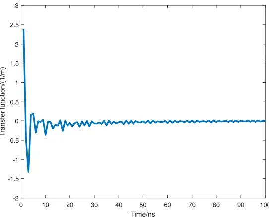
results of the antenna factor are shown in Fig. 1. The time-domain transfer functionh0(t) of the bicone

antenna is calculated by using (3)∼(5) and shown in Fig. 2.

3. CALIBRATE EMP SENSOR WITH BICONE ANTENNA

The calibrated bicone antenna is regarded as a standard antenna during calibrating an EMP sensor, which is a small monopole active sensor. The induced voltage ﬁelds of the calibrated bicone antenna and the EMP sensor, which are placed in a same point successively, are tested and recorded as u0(t)

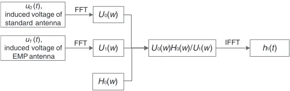
and u1(t), respectively. In frequency domain, they are demoted as H0(w) and H1(w). Supposed H1(w) is the magnitude spectrum of the EMP sensor, obviously, U1(w)H1(w) = U0(w)H0(w),

because these two antennas are placed at the same testing point and in same impulse ﬁeld. Hence,

(3)

20 50 100 150 200 250 300 Frequency/MHz

2 3 4 5 6 7 8 9 10

Antenna Factor/(1/m)

Fitted Antenna Factor

Measured Antenna Factor

Figure 1. Measured and ﬁtted antenna factor curve of a bicone antenna.

0 10 20 30 40 50 60 70 80 90 100 Time/ns

-2 -1.5 -1 -0.5 0 0.5 1 1.5 2 2.5 3

Transfer function/(1/m)

Figure 2. Time-domain transfer function of a bicone antenna.

4. ESTIMATING UNCERTAINTY FOR EMP SENSOR CALIBRATION

Now, we concentrate on the uncertainty of the EMP sensor calibration. In the above mentioned calibration system shown in Fig. 3, the factors that aﬀect the uncertainty include i) Repeatability of measurement of pulse amplitude u0(t) and u1(t). ii) Inhomogeneity of the measured ﬁeld. iii)

(4)

u0(t), induced voltage of standard antenna

u1(t), induced voltage of

EMP antenna

U0(w)

U1(w)

H0(w)

U0(w)H0(w)/U1(w) h1(t) FFT

FFT IFFT

Figure 3. Sensor time domain calibration data processing diagram.

the following formula [10]. For FFT,

uR(k) = ⎧ ⎨ ⎩

√

N umax k= 0

N

2 umax k= 0

(6)

where umax is the maximum uncertainty of all points, and N is the number of sequence points. For

IFFT,

ux = ⎧ ⎪ ⎪ ⎨ ⎪ ⎪ ⎩ 1

N uR n= 0

1 2N(u

2

R+u2I)umax n= 0

(7)

whereuRanduIare the known uncertainties of real and imaginary parts in the frequency domain. Given

that the uncertainties ofU0(w),H0(w) and U1(w) are expressed asuU0,uH0 anduU1, respectively, the

total uncertain of H1(w) may be denoted as [11],

u2_H1=c21u2U0+c22u2H0+c23u2U1 (8)

where, ⎧ ⎪ ⎪ ⎪ ⎨ ⎪ ⎪ ⎪ ⎩

c1 = H_U₁0₍(_ww₎)

c2 = U_U0₁(₍w_w)₎

c3 = U0(W_U2)H0(w) 1(w)

.

The uncertainty of antenna factor of the standard bicone antenna for calibration is 1.55 dB and

k = 2. At the same time, the uncertainty for each of the two measurement voltages, u0 and u1, is

estimated to be 2 dB. By calculation, the maximum uncertainty for h(t) is 2.79 dB if N = 16384.

5. COMPARE TIME-DOMAIN FUNCTION WITH TEM CELL CALIBRATION

To the best of our knowledge, there is no uniform standard that can be used for comparing the accuracy of the EMP calibration methods. In our investigation, we verify the presented method with TEM cell calibration. In the TEM cell, the electric field strength is known, and its time domain voltage waveform is measured firstly using a small monopole active sensor, whose EMP amplification transfer factor is 51.41. Fig 4(a) shows the measured voltage waveform of the small sensor received in time domain, and Fig. 4(b) is the field waveform which is obtained by the voltage multiply by the transfer factor directly. It can be seen from the figure that the peak-peak amplitude of the tested field EP P T = 14.4 V/m. We regard the results as a reference since it is calibrated.

After that, the small monopole active sensor is replaced by another wideband antenna whose antenna factor is unknown. It is worth mentioning that all other testing environments, including the position of two antennas, signal source, testing devices and transmission lines, remain unchanged. Then, the electric ﬁeld strength is reconstructed with the method mentioned earlier. The calculated result is shown in Fig 5, which exhibits that the peak-peak amplitude of the reconstructed ﬁeld is

EP P R = 15.4 V/m. We see that the diﬀerence between the reconstruction result and the calibrated one

(5)

0 50 100 150 200 250 T/ns

-0.2 0 0.2

U/V

0 50 100 150 200 250

T/ns -10

0 10

E/(V/m)

(a)

(b)

Figure 4. Small sensor measurement of the digital voltage waveform and ﬁeld waveform corrected by transfer factor.

0 50 100 150 200 250

T/ns

-10 -5 0 5 10

E/(V/m)

Figure 5. Field waveform as corrected by the time domain transfer function.

6. CONCLUSIONS

The electromagnetic pulse fieldE(t) can be measured correctly using the presented calibration method based on the convolution theorem. Obtainingh(t), the time-domain transfer function of the wideband antenna, from its complex antenna factor is a vital step, since E(t) =h(t)∗u(t). The induced voltages of wideband antenna or sensor under calibrating and standard antenna are tested firstly. Then, both voltages in time domain are transformed to frequency domain with FFT. Together with the magnitude spectrum of antenna factor of the standard antenna, the magnitude spectrum of the sensor is calculated. The phase spectrum of the antenna factor with known magnitude spectrum is reconstructed with Hilbert transform. The advantages of the calibration method include i) Frequency domain antenna factors of UWB antennas can be converted into time domain transfer function for measuring EMP field. ii) During calculating the time domain transfer function, the TEM or GTEM cell is not a necessary apparatus, only the FD antenna factor is need. iii) The size of the sensor or antenna under calibrating is not constrained to the size of standard EM field environment.

REFERENCES

1. IEC 61000-4-33-2005 Electromagnetic compatibility (EMC), Part 4-33: Testing and measurement techniques. Measurement methods for high-power transient parameters test equipment.

2. Shi, L. H., B. H. Zhou, and B. Q. Tao, “A discrete transfer function model for the time-domain calibration data of EMP sensors,” Proc. 13th Int. Zurich Symp. Electromagn. Compat., 149–152, Zurich, Switzerland, 1999.

3. Rubinstein, M., J. L. Bermudez, V. Rakov, F. Rachidi, and A. Hussein, “Compensation of the instrumental decay in measured lightening electric ﬁeld waveforms,” IEEE Trans. Electromagn. Compat., Vol. 54, No. 3, 68–688, 2012.

(6)

5. Ma, R., L. Shi, Z. Huang, and Y. Zhou, “EMP signal reconstruction using associated-hermite orthogonal functions,”IEEE Trans. Electromagn. Compat., Vol. 56, No. 5, Oct. 2014.

6. Srgel, W., F. Pivit, and W. Wiesbeck, “Comparison of frequency domain and time domain measurement procedures for ultra wideband antennas,”2003 Antenna Measurement and Techniques Association (AMTA) Conference, 2003.

7. Lawton, R. A., S. M. Riad, and J. R. Andrews, “Pulse and time-domain measurements,”Proceedings of the IEEE, Vol. 74, No. 1, 77–81, 1986.

8. Tesche, F. M., “On the use of the Hilbert transform for processing measured CW data,” IEEE Trans. Electromagn. Compat., Vol. 34. No. 3, 259–266, 1992.

9. Oppenheim, A. V. and R. W. Schafer,Discrete-Time Signal Processing, Prentice Hall, 2009. 10. Yu, Y. and M. Liu, “Research on the uncertainly of transition duration of broadband sampling

oscilloscope based on nose-to-nose technology,” ACTA Metrologyica Sinica, Vol. 28. No. 1, 81–84, 2007.