Compressionion of pulse code modulation signal using type IV discrete cosine transform based on the mp3 model

(1)

USING TYPE IV DISCRETE COSINE TRANSFORM BASED ON

THE MP3 MODEL.

BY:

ANDREW YOTUI CHEPYEGON (B.Sc) REG NO I56/CE/11000/2006

A Thesis Submitted in Partial Fulfillment of the Requirements for the Award of the Degree of Master of Science (Electronics and Instrumentation) in the School of Pure and Applied Sciences of Kenyatta University.

(2)

ii DECLARATION

This study is my original work and has not been presented for the award of a degree or any other award in any other University.

Andrew Yotui Chepyegon Department of Physics Kenyatta University

Signature……….. Date……….

This thesis has been submitted with our approval as University supervisors.

University Supervisors

Dr Willis Ambusso Signature………. Date……….

Department of Physics Kenyatta University

Dr Mathew Munji Signature………. Date……….

(3)

iii DEDICATION

(4)

iv

ACKNOWLEDGEMENT

(5)

v

ACRONYMS AND ABBREVIATIONS

AIFF Audio Interchange File Format

CD Compact Disc

DBA Digital Broadcast Audio

DCT Discrete Cosine Transform

FFT Fast Fourier Transform

IMDCT Inverse MDCT

JPEG Joint Photograph Expert Group MDCT Modified Discrete Cosine Transform MDST Modified Discrete Sine Transform

MP3 MPEG-1 Audio Layer III

MPEG Motion Picture Expert Group

MUSICAM Masking Pattern Adapted Universal Subband Integrated Coding and Multiplexing

ODG Objective Difference Grade

PEAQ Perceptual Evaluation of Audio Quality

PCM Pulse Code Modulation

PQF Polyphase Quadrature Filter.

QMF Quadrature Mirror Filter

RIFF Resource Interchange File Format

SDG Subjective Difference Grade

SNR Signal to Noise Ratio

TDAC Time domain aliasing cancellation

(6)

vi

Table 4.1: Compression percentages for audio signals at a sampling rate of 32000Hz ... 49 Table 4.2: Compression percentages for audio signals at a sampling rate of 41000Hz ... 49 Table 4.3: Compression percentages for audio signals at a sampling rate of 48000Hz ... 50 Table 4.4: Compression ratios for MP1, MP2 and MP3 compression techniques

for audio signals at a sampling rate of 44100Hz ... 51 Table 4.5: Listening Tests Grading Scale based on ITU-R BS.1284 standard

ranging from 1.0 to 5.0. ... 53 Table 4.6: Listener satisfaction survey questionnaire. ... 54 Table 4.7: Table showing comparrisons between the test results of the study,

with the ITU-R BS.1284 grading system. ... 54 Table 4.8: SDG description... 59 Table 4.9: Objective Difference Grade (ODG) scores for ten audio samples

(9)

ix LIST OF FIGURES

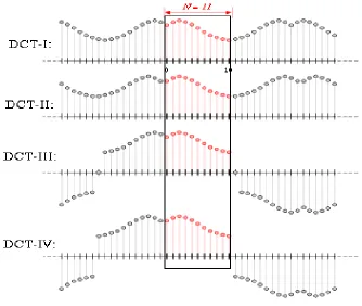
Figure 1.1: Illustration of the implicit even/odd extensions of DCT input data, for N=11 data points (rectangular region), for the four most common

types of DCT ... 4

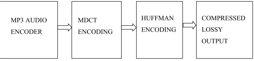
Figure 1.2: Diagram showing the MP3 Encoder after attaching an MDCT encoder. ... 5

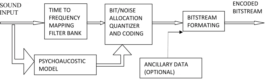
Figure 1.3: Basic MP3 Audio encoder diagram illustrating how the different components are connected. ... 6

Figure 2.1. Block diagram showing the two main parts to the PEAQ algorithm ... 15

Figure 3.1: The coding flow diagram. ... 17

Figure 3.2. Generic perceptual audio coder. ... 19

Figure 3.4. MP3 Encoder Structure showing specific activities performed during audio encoding of the audio encoding chain, which provides a generalized overview of the flow of the coding involved in the development of the encoder in this project. ... 23

Figure 3.5: The Four parts of an MP3 frame . ... 35

Figure 4.1: The MDCT project Front panel. ... 45

Figure 4.2: The recording interface ... 46

Figure 4.3: File compression summary window. ... 48

Figure 4.4: Audio1_32.wav waveform. ... 56

Figure 4.5: Audio1_32.mp3 waveform. ... 56

(10)

x

LIST OF LISTINGS

Listing 3.1: Part of the code for capturing the PCM signals ... 21

Listing 3.2: Setting the coefficients for the MDCT encoding. ... 25

Listing 3.3: The MDCT Filtering... 26

Listing 3.4: The MDCT sub band Filtering ... 26

Listing 3.5: The Quantization process ... 30

Listing 3.6: The Huffman table selection criteria. ... 31

Listing 3.7: The frame Header format coding. ... 36

Listing 3.8: The Side information coding ... 40

(11)

xi ABSTRACT

(12)

1

CHAPTER ONE

INTRODUCTION

1.1 Background to the study

Data compression can be classified as either lossless or lossy (Brandenburg and Stoll, 2009). In a lossless compression, an exact copy of the original signal after decompression is produced while in the lossy compression, the original signal can no longer be reproduced. Lossless compression can successfully be applied in situations where there is plenty of data redundancy. It is easier to apply techniques like run-length suppression or Lempel–Ziv (LZ) compression. An example of a compression which maintains its original file is the ZIP file format. Lossless data compression is effective on several types of files (Jacaba, 2001). Lossless compressing of audio through this method is not as effective due to the fact that the information therein is less redundant (William, 1998). For this reason, we then prefer the lossy or perceptually lossless compression (Jacaba, 2001). Of the existing lossy encoding techniques, the Motion Picture Experts Group (MPEG)-1 Audio Layer III (MP3) standard, stands out as the most efficient and widely applied. The amount of data required to represent the audio signal recorded as PCM is tremendously reduced while its perceptual quality is still a good reproduction of the original uncompressed audio. An MP3 file with a setting of 128 kbit/s normally results in a file which is about 1/11 the size of the original audio file. Higher or lower bit rates can be used for MP3 files, with higher or lower output quality (Chiariglione and Leonardo, 2009).

(13)

2

in areas like satellite communications. Examples are DBS TV’s, TATA SKY, dish television network. They use MPEG-4, MPEG-1, MPEG-2 and MPEG-DASH. The compression of Speech has a streaming method so dynamic and adaptive over HTTP (DASH) technology. The technology is also being widely applied in cellular technology which includes mobile telephony as well as Voice over IP (Ramírez, 2008).

1.2 Theoretical Framework

The MPEG 1 standard was generally used with techniques and methods for compressing video and audio. MP3 is part of the MPEG 1 audio standard. Specifically, MP3 is “Layer 3” of MPEG 1. There are three 'layers' defined for MPEG 1 audio, with each layer being more complex than the previous and with each providing improved results. The layers are backwards-compatible, and therefore any software or hardware which can play (or 'decode') Layer 3 audio should consequently be able to decode both Layers 1 and 2 (Paul, 2000).

MP3 employs the “Discrete Cosine Transformation” (DCT) mathematical algorithm to compress signals. It takes a finite number of data points in sequence and in terms of a sum of cosine functions at different frequencies. Cosine functions use fewer functions than sine functions and for that reason are generally used to approximate a typical signal. For differential equations as well, the cosines express boundary conditions of choice (Narasimha and Peterson, 1978).

(14)

3

sample. According to Literature, the DCT hase eight types of transforms, four of which are commonly used (Wen-Hsiung et al., 1977).

The type-II DCT transform is the most common variant, and is often simply reffered to as “the DCT”. The inverse, which is the type-III DCT, is also called “the inverse DCT” or simply “the IDCT” correspondingly. The Sine counterparts are the discrete sine transforms (DST), which are equivalent tos DFTs which have both real and odd functions, and the type IV DCT also known as the modified discrete cosine transforms (MDCT), which is a transform based on a DCT of overlapped data (Johnson, 1987).

The MDCT, which is a lapped (Overlapping basically helps in avoiding distortions stemming from frame boundaries), is a Fourier transform which is based on type-IV discrete cosine transform (DCT-IV). It uses half as many outputs as inputs contrary to the same number as in other transforms, giving it a high compaction of energy. This is the main characteristic of MDCT that made it quite justifiable to apply as part of the lossy compression in our coder. The MDCT is a linear function F: R2N RN where R denotes the set of real numbers. The 2N real numbers x0, ..., x2N-1 are actually the number of samples that were taken from the input signal (basically the MP3 outputs), and which were then transformed into the N real numbers X0, ..., XN-1 ( the outputs of the MDCT transformation) according to the formula (Johnson et al., 1987):

Xk= 1.1

where k is any of the 1 to N outputs of the MDCT.

(15)

4

cancellation. The boundary conditions in a subtle way are the reason behind for the high energy compaction associated with the DCTs, and its usefulness is in image and audio compression. This is because the boundary behavior affects how much convergence there is in any Fourier-like series.

Figure 1.1: Illustration of the even/odd extensions of DCT data, for N=11 data points (rectangular region), for the four common types of DCT (types I-IV)(Rao and Yip, 1990) http://en.wikipedia.org/wiki/Discrete_cosine_transform).

The MDCT basically takes samples of the outputs of the MP3 encoder and filters them to produce a more compressed signal with a better quality (less artifacts) using a window function given by equation 1.2.

1.2

(16)

5

= 0 and 2N boundaries by ensuring that the function smoothly approaches zero at these points.

Recording equipment such as microphones and guitars, produce a wide range of audio resolutions most of which the human ear cannot perceive. When recorded in high fidelity, sound stores a lot of audio data that are inaudible, and by eliminating them, the final resulting audio sound will be indistinguishable from the originaly recorded. The MP3 format by this concept can attain compressions of ratios of up to 1:24. However, MPEG-1 standard for audio compression does not include a strict specification for an MP3 encoding (Davis, 1995). Any developer or researcher keen on implementing the standard is expected to devise own unique algorithms for removing portions of the information in the PCM audio. This consequently has led to many different MP3 encoders, each producing files of varying or different quality. This project did attach a Modified Discrete Cosine Transform (MDCT) encoding coupled with Huffman encoding to produce a lossy compression with better quality than pure MP3. The Huffman encoding was applied to reduce any redundancies that might exist within the compressed outputs. The flow diagram is as shown in figure 1.2.

The four main components of MP3, namely filterbank, psychoacoustics, quantization and bitstream formatting are shown in figure 1.3.

MP3 AUDIO ENCODER

MDCT ENCODING

HUFFMAN ENCODING

COMPRESSED LOSSY

OUTPUT

(17)

6 1.3 Statement of the research problem

MP3 being one of the commonly used methods for compressing audio by removing irrelevant data from some recording, employs mathematical algorithms like the “Fast Fourier Transform” (FFT) or “Discrete Cosine Transform” (DCT) to achieve this (Peterson, 1978). Depending on the choice of algorithm chosen, the MP3 standard gives the freedom of how the irrelevant data in an input audio signal can be removed (Brandenburg and Stoll, 1987). The standard simply gives an outline of the necessary techniques and specifies the format for encoding the audio. MP3 is ambiguous and poorly written as it gives no details of implementation in some places. No emphasis is placed on the efficiency of computation. A new MP3 decoder is therefore a greater task than one would otherwise expect. Furthermore, the implementation of the MP3 technique during signal compression produces outputs accompanied by signal distortions (Schuller, 1998). In this study, a Modified discrete Cosine transform compression technique for sound optimization (MDCT) filter bank that adaptively switches between 128 and 1024 bands is implemented using Visual Basic.NET. The MDCT was used to double the number of frequency bands available for coding signals and which expectedly contributed to increased coding gain of this method.

SOUND

INPUT TIME TO

FREQUENCY MAPPING FILTER BANK

BIT/NOISE ALLOCATION QUANTIZER AND CODING

BITSTREAM FORMATING

PSYCHOAUCOSTIC MODEL

ENCODED BITSTREAM

ANCILLARY DATA (OPTIONAL)

(18)

7 1.4 Objectives

1.4.1 General Objective

The general objective of this study was to design an application that utilizes the Modified Discrete Cosine Transform (MDCT) techniques to compress audio files based on the MP3 standard.

1.4.2 Specific Objectives

(i). To create Visual Basic software components which would divide raw audio input into small Samples, i.e., the signal was to be made to pass into a time-frequency mapping filter bank which would divide it into sub bands.

(ii). To apply Psychoacoustic modeling to the sound samples. The concepts of masking and thresholds were to be utilized to discard data that was inaudible. (iii). To quantize the output samples and then perform an MDCT filter on the output. (iv). To apply both Subjective and Objective evaluation techniques to establish

whether the MDCT encoding compromises on output signal quality.

1.5 Rationale/Justification of the Study

(19)

8

CHAPTER TWO

LITERATURE REVIEW

2.1 Introduction

The MPEG-1 Audio Layer III (MP3) format of signal compression used in encoding audio data uses a lossy compression. It is based on acoustics and psychoacoustics which considers the way the human ear interprates signals. This phenomenon is also known as the perceptive behavior of the human ear. MPEG is the official standardization by a committee formed under the International Electro technical Commission (IEC) and the International Standards Organization (ISO), for the sole purpose of developing international standards which guides the efficient encoding of video for motion picture and high quality and fidelity audio. In 1993, the MPEG committee published the MPEG standard in the form of the document ISO/IEC 11172. It therefore set out a common standard for the coding of video or moving pictures and the associated audio signals for digital transmission and storage in digital media at rates of up to about 1.5 Mbit/Second, and it was named the MPEG 1 standard (Paul, 2000).

(20)

9

are as a reason of how the processing of signals in the brain takes place. It therefore means that these masked sounds can effectively be filtered off without affecting the quality of the final audio signal, thus justifying why MP3 standard, which is a lossy compression technique was considered in this study as a basis for the MDCT compression.

Audio Compact Disks (CDs) use the popular waveform (WAV) format, which is uncompressed (Davis, 1995). The WAV format falls in many categories one of which is the Pulse Code Modulation (PCM) which is the commonly accepted MP3 input during enoding. The WAV file size depends on the rate of which it is sampled. As an example, an 8-bit mono WAV sampled at 22,050 Hertz (Hz) would take 22,050 bytes per second. A 16-bit stereo WAV file which has been sampled at the rate of 44.1 kilohertz (kHz) would take 176,400 bytes per second (this has been calculated as 44,100 per second * 2 bytes * 2 channels). Calculations of a one minute of an audio file of CD-quality takes a storage space of 10 MB. It is therefore necessary to find methods and algorithms for reducing huge requirements in data storage of such files. MP3standadrd is one of the methods mostly used for this purpose (Jacaba, 2001).

2.2 Lossless and Lossy coders

(21)

10 2.3 Existing Coders and Standards

Several implementations of perceptual coders exist in commercial use. Those considered to be top-of-the-line include Sonys ATRAC, which is used in the MiniDisc system. MPEG-1 Layer I, II and III standards are the other well known examples that implement perceptual coding (Brandenburg and Stoll, 1987). MPEG-2 Advanced Audio Coding (AAC) and Dolby's AC-3 (Bosi et al., 1997). The differences in the compression technique between the many coders are in the way they model the human ear and the type of subband coding used. The general problem in these coders is how to handle certain signal artifacts, which are noticeable distortion of audio media caused by the application of lossy approach in the compression of data. Currently, the MP3 standard is the format commonly used for audio streaming or storage in consumer products. It is also the de facto standard for digital compression of audio as well as the transfer and playback on most digital audio players (Chiariglione and Leonardo, 2009).

2.3.1 Subband Coders

Subband splitting or filtering of a signal is a method used over and over to refine bands in a filter tree (Princen et al, 1997). The splitting of a 20000Hz signal for instance, would be split as:

0 – 20000 Hz → 0 - 10000 Hz, 10000 - 20000 Hz

0 - 10000 Hz → 0 - 5000 Hz, 5000 Hz - 10000 Hz

The coder in this way can divide the input audio data into several equal bands, where each of which a quantizer, adapted to the masking threshold, is finally applied.

(22)

sub-11

sampled using a factor of 2. To reconstruct the signal, the two bands are again up-sampled and filtered using the G's. The output expression for is as shown in

equation 2.1;

2.1

Aliasing cancellation for the filters G0(w), and G1(w), is obtained by the requirements of equations 2.2 and 2.3 (Princen et al, 1997).

2.2

2.3

Optimally,

2.4

With these equations, a good reconstruction is achieved. In most coders, the filters used are Quadrature Mirror Filters (QMF). They manage to perform distortion or aliasing eradication by choosing F1 such that it is the mirror image of F0 (around ᴨ/2):

2.5

(23)

12 2.3.2 MPEG-1, Layer I and II

The ISO MPEG-1 coding standard has layers I, II and III all of which differ in coding and psychoacoustic models (Davis, 2005).

Both Layers I and II use a QMF filter bank of order 511, and which has a 96 dB rejection of side-lobes and also has a steep transition of pass-to-stop-band. The filter bank splits the the audio input into 32 sub-bands.

MPEG layer III uses the psychoacoustic model which consists of a 512 point Fast Fourier Transform (FFT), from which a masking threshold is calculated using equation 3.2 shown in chapter 3 section 3.3.2. Here, the maximum values of the spectrum are considered as components which influence the tonal portion of the signal and are therefore treated differently from the noise components. To produce a masking threshold, both the noise and the tonal masking thresholds are added. A linear quantizer is used together with the masking threshold to achieve the required performance in the rate-distortion in each sub-band. Eventually each sub-band will then have the same noise-to-mask-ratio and the bits add up to the appropriate bit-rate. The quantized sub-band is fixed-length encoded rather than running length encoded.

2.3.3 Wavelet Coders

(24)

13

2.4 Modified Discrete Cosine Transform (MDCT)

It is also referred to as MPEG-2 AAC and is designed to take the place of the MP3 compression technique. In MDCT, the input audio data is initially split using a Polyphase Quadrature Filter (PQF) into four uniform subbands (Bosi et al., 1997). An individual gain is then transmitted as side information for each subband. The subband data controlled by the gain is then transformed using an MDCT whose frame length is 256 (for transient conditions the length is 32). The sine window of equation 1.2 in chapter one is used to smothen the boundary artifacts for the MDCT. The windowing function has different spectral characteristics, which are suitable for a variety of signals. For conditions which are transient in nature, a shorter window is used for improved resolution of time. The coefficients of the MDCT are computed from two preceding frames, using a separate Least Mean Square (LMS) predictor adapted for every frequency band. This method when applied to stationary signals improves coding efficiency (Bosi et al., 1997).

The MDCT transformation is understood on the basis of the knowledge of Time Domain Aliasing Cancellation (TDAC) and is also a linear orthogonal transform which is lapped for better energy compaction (Princen and Bradley, 1986; Princen et al., 1987).

(25)

14

It is very effective in removing blocking artifacts that would have otherwise been easy to detect between the transform blocks. The definition of MDCT is summarized in equation 2.6, (Sporer et al, 1997).

2.6

The corresponding IMDCT is shown in equation 2.7.

2.7

where f(x), is the window function explained in equation. 1.2.

In this coder, the MDCT transformation was achieved using frames whose lengths are 512, producing 256 samples which were then used consecutive blocks.

2.5 Perceptual Evaluation of Audio Quality (PEAQ)

The International Telecommunications Union (ITU) proposes a standard that can be used to asses the quality of audio files after has undergone some transformation. This standard which as of the writing of this thesis was the only method used for assessing audio quality is known as the Perceptual Ealuation of Audio Quality (PEAQ). It is mostly used while developing codecs and networks and also for testing multimedia devices for audio playback quality. ITU-RBS.1387 standardized the PEAQ during 1998–2001 (Campbell

(26)

15

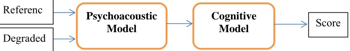
based algorithms which are designed to facilitate objective assesment of the quality of audio devices, computer networks and digital systems. The one such algorithm is the PEAQ which essentially models the behavior of the human ear. In other words it is designed based on the psychoacoustic principles of the human auditory system. It ia designed to maintain an acceptable level of audio quality despite a reduction in the number of bits of an audio signal. PEAQ consists of two parts namely the psychoacoustic model and the cognitive model. The overview is shown in figure 2.1. In figure 2.1, the original undistorted signal is used as the reference. The degraded input represents the distorted output test signal that needs assessment. The final scores are given as values in the range 0 to -4.

Figure 2.1: Block diagram showing the two main parts to the PEAQ algorithm (Campbell, 2009).

There are two vesrions of PEAQ: the basic version and the advanced version. The former is intended for those applications requiring high processing speed, and the latter is for applications requiring highest accuracy (Vanam, 2005).

The PEAQ basic version utilizes an FFT-based psychoustic model. The advanced version on the other hand uses the FFT-based rmodel together with a filterbank-based model of the human ear. The concept of sound masking is implemented with the FFT-based ear model, and the concept of internal representations comparisons is implemented using the filterbank-based ear model. There are eleven model output variables (MOV) jn

Psychoacoustic Model

Cognitive Model Referenc

Degraded

(27)

16

(28)

17

CHAPTER THREE

RESEARCH METHODOLOGY

3.1 Coding:

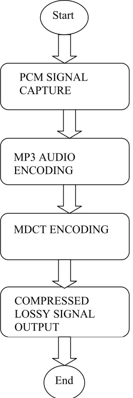
The study was code intensive. Part of the Code was purely for capturing raw sound signal from a microphone or sound card, in form of PCM for storage before being compressed further using MP3 and finally MDCT. The code modulation followed the steps shown in figure 3.1.

COMPRESSED LOSSY SIGNAL OUTPUT

MP3 AUDIO ENCODING

PCM SIGNAL CAPTURE

MDCT ENCODING Start

End

(29)

18 3.2 Algorithm:

1. Read an uncompressed audio format file, PCM, which is usually stored in a waveform (WAV) file on Windows or in an audio interchange file format (AIFF) file on Mac OS. Windows waveform (WAV) was used in this study.

2. Use Convolution filters to divide the input signal into subbands containing 32 critical bands.

3. Compute the masking values for every band due to the bands in its neighbourhood using the results from step 2.

4. No encoding for a band whose power is below the masking threshold.

5. Determine how many bits are required to represent the coefficient with values that will ensure noise introduced by quantization is no more than the effects of masking.

6. Create an MDCT Object to format the output of previous steps. 7. Run MDCT object on all blocks read from Step 6 above. 8. Run the quantization function on all blocks.

9. Finally save the compressed signal in file. 10.Play the audio signal.

3.3 Algorithm description and Analysis

(30)

19

Painter and Spanias (2000) describe that the coder in figure 3.2, creates segments of quasistationary frames from the input audio s (n) which range from 2 to 50 ms in a given time. Next the analysis block for the time-frequency mapping computes an estimation of the temporal and spectral components found in each given frame. A mapping of these components to the properties used for analysis of the behavior of the human auditory system and then finally the time to frequency mapping parameters that will be used for quantization and eventually encoding are extracted.

The block responsible for psychoacoustics which is also called the psychoacoustic block permits for the quantization and consequently the encoding block to take advantage of information that cannot be perceived in the time to frequency set of parameter. The remainders of the redundancies are ususlly removed through the process of lossless entropy coding techniques.

Parameters Parameters

Time/Frequency

Analyisis Quantization and encoding

Entropy (lossless) Coding S(n)

Psychoustic Analyisis

Bit Allocation

Side Info Masking Thresholds

(31)

20 3.3.1 PCM Signal capture

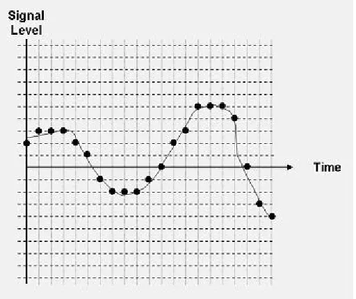
The Audio signal represented by sine waves of varying frequencies, is initially in an Analog format, meaning that it is a continuous signal. The human ear has the ability to percieve frequency nominally in the range of 20 to 20,000 cycles/second (Hertz or Hz). To Store sound in a digital format, it is required that the sound wave which is continuous be converted to a group of samples that can then be represented by a train of zeros and ones.

Conversion of the signals from Analog to digital formats was accomplished by sampling the analog signal using a microphone, after which the signals were converted to equivalent voltage levels. The voltage or signal levels were converted into digital bits by use of a coder-decoder or codec to a numeric value using a pulse code modulation (PCM) method. The code in listing 3.1 shows the section of the code that was used to capture the raw uncompressed audio signal.

(32)

21 Figure 3.3: Simple Pulse Code Modulation

For a good sampling, analog signals need to be recorded at a sampling frequency which is twice the highest frequency value of the input signal according to Nyquist sampling theory; this is so that the original signal can be reproduced to a near resemblance from the samples. Applications of Music audio always assume the full wave spectrum of the human ear i.e from 20Hz to 20000Hz and generally use a 44.1 k (Painter, 2000).

Listing 3.1: Part of the code for capturing the PCM signals

PrivateSub StartOrStopRecord(ByVal StartRecording AsBoolean) ' Starts or stops the capture buffer from recording

Writer = New BinaryWriter(WaveFile) If Recording = StartRecording Then ' Create a capture buffer

(33)

22 Recording = True

applicationBuffer.Start(True) Else

' Stop the buffer

applicationBuffer.[Stop]() RecordCapturedData()

Writer.Seek(4, SeekOrigin.Begin)

' Seek to the length descriptor of the RIFF file. Writer.Write(CInt(SampleCount + 36))

Writer.Seek(40, SeekOrigin.Begin) Writer.Write(SampleCount)

Writer.Close() Writer = Nothing WaveFile = Nothing 'Recording = False Capturing = False 'NotificationEvent.Set() EndIf

EndSub

(34)

23

occupy nearly 10.6 MB (1,411,200 bits * 60 seconds / 8 bits = 10,584,000 bytes). In essence, audio files are made smaller by compressing them using a several available techniques. A quick method for doing so is to reduce the number of channels from two to one or to reduce the sampling rate to a lower value than 44.1 KHz, in some cases to as low as 11 kHz. Any of the chosen solutions will in some way reduce the quality of the sound. Here we used the Fast Fourier Transform (FFT) block to transform granules of 576 samples to the frequency domain using Fourier Transform.

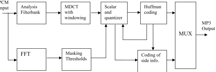
3.3.2 MP3 audio encoding

The MP3 encoder has the structure of figure 3.4 (Pan, 1995):

Figure 3.4 is a refined version of figure 1.2. It presents specific activities for each section

The PCM input data, after been sampled was stored in disk as uncompressed file with a .wav extension. The file was then split into frames of 1152 samples each. Each of the frames was further divided into two granules of 576 samples per frame. The frames were then processed by the FFT block for correlation before finally passing through the analysis filterbank.

Scalar and quantizer

Huffman coding

Coding of side info.

MUX

Masking Thresholds FFT

MDCT with windowing Analysis

Filterbank PCM

Input

MP3 Output

(35)

24

The main function of the FFT algorithm was to reduce the number of computations for N points from 2N2 to N log N, where the log is in base-2 logarithm. Fourier transforms that use base-4 and base-8 are normally optimized code, which can be 20-30% faster than base-2 FFTs. The FFT function itself is given by equation 3.1 (Painter, 2000).

3.1

There first term on the right hand side of equation 3.1 above represents the even coefficients while the second term represents the Odd coefficients of the samples within the signal.

The results obtained from applying the FFT, which are now in the frequency domain, were used together with a psychoacoustic model to determine the masking thresholds for all frequencies integrated within the audio signal. The masking thresholds formula is given by equation 3.2 (Terhardt, 1979).

3.2

where f represents frequency (Hz) and dB is the unit of threshold.

3.3.3 MDCT

(36)

25

Higher frequency resolution was achieved by the use of DCT and the control of the pre-echo (Painter, 2000). The application of MDCT to every time frame of the given subband samples splits the 32 subbands into 18 smaller and more refined subbands, and a granule with a total of 576 frequency lines is thus created.

To reduce the noise caused by the boundaries of the signal in the spatial domain before performing the MDCT, each subband signal had to be windowed with the sine function shown in equation 1.2. The MDCT is performed on blocks that are windowed and overlapped by 50%. Listing 3.2 shows how the coefficients of the MDCT are determined and listing 3.3 and 3.4 are the MDCT filtering and sub band filtering methods respectively.

Listing 3.2: Setting the coefficients for the MDCT encoding. PrivateSub mdct_initialise()

Dim i, m, k AsInteger'N; Dim sq AsDouble

' prepare the aliasing reduction butterflies For i = 7 To 0 Step -1

sq = Math.Sqrt(1.0 + Math.Pow(c(i), 2)) ca(i) = c(i) / sq

cs(i) = 1.0 / sq Next i

For i = 35 To 0 Step -1

(37)

26 Next i

'N = 36;

For m = 0 To 17 For k = 0 To 35

cos_l(m, k) = Math.Cos((Math.PI / (72)) * (2 * k + 19) * (2 * m + 1)) / (9) Next k

Next m EndSub

Listing 3.3: The MDCT Filtering

PrivateSub mdct(ByVal SamplesIn() AsDouble, ByVal SamplesOut() AsDouble) Dim k, m AsInteger

For m = 18 To 0 Step -1

SamplesOut(m) = win(35) * SamplesIn(35) * cos_l(m, 35) For k = 35 To 0 Step -1

SamplesOut(m) += win(k) * SamplesIn(k) * cos_l(m, k) Next k

Next m EndSub

Listing 3.4: The MDCT sub band Filtering

Private Sub mdct_sub(ByVal sb_sample(,,,) AsDouble, ByRef mdct_freq(,) AsDouble, ByRef side_info() As side_info_t)

(38)

27 ReDim mdct_freq(2, samp_per_frame2) Dim mdct_enc(2, 32, 18) AsDouble

'mdct_enc(2, 32, 18) = mdct_freq(2, 32, 18) Dim ch, gr, band, k, j AsInteger

Dim cod_info() As gr_info Dim mdct_in(36) AsDouble Dim bu, bd AsDouble For gr = 0 To gr < 2

For ch = config.wave.channels To 0 Step -1

'cod_info = (gr_info*) &(side_info.gr(gr).ch(ch)) ' Compensate for inversion in the analysis filter For band = 32 To 0 Step -1

For k = 18 To 0 Step -1

If ((band And 1) And (k And 1)) Then sb_sample(ch, gr + 1, k, band) *= -1.0 EndIf

Next k Next band

' Perform imdct of 18 previous subband samples + 18 current subband samples

For band = 32 To 0 Step -1 For k = 18 To 0 Step -1

(39)

28

mdct_in(k + 18) = sb_sample(ch, gr + 1, k, band) Next k

mdct(mdct_in, mdct_enc(gr, ch, band), 0) Next band

' Perform aliasing reduction butterfly For band = 31 To 0 Step -1

For k = 8 To 0 Step -1

bu = mdct_enc(gr, ch, band, 17 - k) * cs(k) + mdct_enc(gr, ch, band + 1, k) * ca(k)

bd = mdct_enc(gr, ch, band + 1, k) * cs(k) - mdct_enc(gr, ch, band, 17 - k) * ca(k)

mdct_enc(gr, ch, band, 17 - k) = bu mdct_enc(gr, ch, band + 1, k) = bd Next k

Next band Next ch Next gr

' Save latest granule's subband samples to be used in the next mdct call For ch = config.wave.channels To 0 Step -1

For j = 18 To 0 Step -1 For band = 32 To 0 Step -1

(40)

29 Next j

Next ch EndSub

Listing 3.4 shows the portion of the code used to create the overlapping effect of the MDCT whose inputs are 2N and whose outputs are N. It achieves this by dividing the inputs of the signal into four blocks of size N/2 each. If these inputs are shifted by N/2 then the end of the N DCT-IV inputs will create a “fold back” according to the signal edge conditions described in equation 3.3 and equation 3.4. Thus, the MDCT of 2N inputs is exactly the same as that of a DCT-IV of N inputs.

3.3

3.4

3.3.4 Compressed signal output formatting

The number of bits required or needed for each critical band to represent the samples so that noise is minimized was determined by use of masking thresholds. Afterwards the psychoacoustic model was used to allocate bits.

(41)

30 Listing 3.5: The Quantization process

Private Sub quantize(ByVal xr() As Double, ByVal ix() As IntPtr, ByRef cod_info As gr_info)

Dim i AsInteger Dim idx AsInteger Dim steps AsDouble Dim dbl AsDouble Dim ln AsLong

steps = Math.Pow(2.0, (cod_info.quantizerStepSize) / 4) For i = samp_per_frame2 To 0 Step -1

dbl = Math.Abs(xr(i)) / steps ln = CLng(dbl)

If (ln < 10000) Then idx = int2idx(ln)

If (dbl < idx2dbl(idx + 1)) Then ix(i) = idx

Else

ix(i) = idx + 1 EndIf

EndIf Next EndSub

(42)

31

bands. According to (Pan, 1995), the process stops depending on when any of the conditions below is met:

a) When the scale factor bands contain less distortions than the accepted value b) The proceeding iteration causes excess amplification for any of the bands. c) The proceeding iteration requires that all values of the scale factor

bands be increased.

The iterations include the Huffman coding since it is needed for determining the number of bits needed for the encoding. Listing 3.6 shows the section of program code that helps choose the specific Huffman values to be used during the quantization process.

After the samples have been quantized, they are Huffman-coded and finally stored in the bitstream with the scale factors and side information.

Listing 3.6: The Huffman table selection criteria.

Function new_choose_table(ByVal ix() As Integer, ByVal begin As UInteger, ByVal ends AsUInteger) AsInteger

'********************************************************************/

' Choose the Huffman table that will encode ix[begin..end] with */

'the fewest bits. */

'**************************************************************/ ix(samp_per_frame2)

(43)

32 max = ix_max(ix, begin, ends)

If (Not max) Then Return 0

EndIf

choice(0) = 0 choice(1) = 0 If (max < 15) Then

' try tables with no linbits */ For i = 14 To 0 Step -1 If ht(i).xlen > max Then choice(0) = i

ExitFor EndIf 'End If Next i

sum(0) = count_bit(ix, begin, ends, choice(0)) SelectCase choice(0)

Case 2

sum(1) = count_bit(ix, begin, ends, 3) If sum(1) <= sum(0) Then

(44)

33 Case 5

choice(0) = 6 EndIf

Case 7

choice(0) = 8 sum(0) = sum(1) EndIf

choice(0) = 9 EndIf

Case 10

choice(0) = 11 sum(0) = sum(1) EndIf

(45)

34 choice(0) = 12

EndIf Case 13

choice(0) = 15 EndIf

EndSelect Else

max -= 15 For i = 15 To 23

If ht(i).linmax >= max Then choice(0) = i

ExitFor'break; EndIf

If ht(i).linmax >= max Then choice(1) = i

(46)

35

sum(0) = count_bit(ix, begin, ends, choice(0)) sum(1) = count_bit(ix, begin, ends, choice(1)) If sum(1) < sum(0) Then

choice(0) = choice(1) EndIf

EndIf

Return choice(0) EndFunction

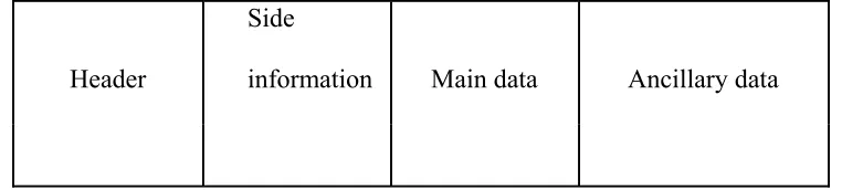
3.3.5 Frame Format

1152 mono or stereo spectral samples samples form part of the frame. These samples are each divided into two granules of 576 samples each as demonstrated in listing 3.4. A further division of each granule produces 32 subband blocks of 18 frequency lines each. The frequency spectrum ranges from 0 to FS/2 (Sampling frequency divided by 2) Hz. ). The frame consists of the header, side information, main data, and ancillary data:

Header

Side

information Main data Ancillary data

Figure 3.5: The Four parts of an MP3 frame (Lagerström, 2001).

(47)

36 Listing 3.7: The frame Header format coding.

Private sub Frame_Header(byval is(SBLIMIT,SSLIMIT) as long , byval xr(SBLIMIT,SSLIMIT) asdouble , _

byref scalefac as III_scalefac_t, byref gr_info As gr_info_s, _ byval ch AsInteger , byref fr_ps As frame_params *) Dim ss, sb AsInteger

Dim cb AsInteger = 0

sfreq = fr_ps.header.sampling_frequency Dim stereo AsInteger = fr_ps.stereo

Dim next_cb_boundary, cb_begin, cb_width, sign AsInteger

' choose correct scalefactor band per block type, initalize boundary If gr_info.window_switching_flag And gr_info.block_type = 2 Then If gr_info.mixed_block_flag Then

next_cb_boundary = sfBandIndex(sfreq).l(1) 'LONG blocks: 0,1,3 Elseif

next_cb_boundary = sfBandIndex(sfreq).s(1) * 3 ' pure SHORT block cb_width = sfBandIndex(sfreq).s(1)

cb_begin = 0

Else

next_cb_boundary = sfBandIndex(sfreq).l(1) ' LONG blocks: 0,1,3 EndIf

(48)

37 For ss = 0 To SSLIMIT - 1

If ((sb * 18) + ss = next_cb_boundary) Then' Adjust critical band boundary If (gr_info.window_switching_flag And (gr_info.block_type = 2)) Then If (gr_info.mixed_block_flag) Then

If (((sb * 18) + ss) = sfBandIndex(sfreq).l(8)) Then next_cb_boundary = sfBandIndex(sfreq).s(4) * 3 cb = 3

cb_width = sfBandIndex(sfreq).s(cb+1) - sfBandIndex((sfreq).s(cb))

cb_begin = sfBandIndex(sfreq).s(cb) * 3 EndIf

ElseIf (((sb * 18) + ss) < sfBandIndex(sfreq).l(8)) Then next_cb_boundary = sfBandIndex(sfreq).l((++cb) + 1) Else

next_cb_boundary = sfBandIndex(sfreq).s((++cb) + 1) * 3 cb_width = sfBandIndex(sfreq).s(cb+1) -

sfBandIndex(sfreq).s(cb)

Else

next_cb_boundary = sfBandIndex(sfreq).s((++cb) + 1) * 3 cb_width = sfBandIndex(sfreq).s(cb+1) -

(49)

38

Else' long blocks

next_cb_boundary = sfBandIndex(sfreq).l((++cb) + 1) EndIf

' Compute overall (global) scaling.

xr(sb, ss) = Math.Pow(2.0, (0.25 * (gr_info.global_gain - 210.0))) ' Do long/short dependent scaling operations.

If (gr_info.window_switching_flag And ( _

((gr_info.block_type = 2) And (gr_info.mixed_block_flag = 0)) Or _ ((gr_info.block_type = 2) And gr_info.mixed_block_flag And (sb >= 2)))) Then

xr(sb,ss) *= pow(2.0, 0.25 * -8.0 * _

gr_info.subblock_gain[(((sb*18)+ss) - cb_begin)/cb_width)) xr(sb,ss) *= pow(2.0, 0.25 * -2.0 * (1.0+gr_info.scalefac_scale) _ * (*scalefac)(ch).s((((sb*18)+ss) - cb_begin)/cb_width,cb)) ' End If

Else ' LONG block types 0,1,3 & 1st 2 subbands of switched blocks * xr(sb,ss) *= pow(2.0, -0.5 * (1.0+gr_info.scalefac_scale) _

* ((*scalefac)(ch).l(cb) _ + gr_info.preflag * pretab(cb))) EndIf

(50)

39 If (iis(sb, ss) < 0) Then

sign = 1 Else sign = 0 EndIf

xr(sb,ss) *= math.pow( convert.ToDouble( abs(iis[sb][ss])), (convert.ToDouble(4.0/3.0)) )

if (sign) xr(sb,ss) = -xr(sb,ss) EndIf

Next Next EndSub

3.3.5.1 Header

The MDCT header based on the MP3 is 4 bytes long and within it is information about the layer type, the bitrate, the sampling frequency and its stereo mode as shown in Listing 3.7. There is also a 12-bit synchronized word used to find the start of a frame in a bitstream especially during playback, or can be used for broadcasting applications (Lagerström, 2001).

3.3.5.2 Side Information

(51)

40

(Lagerström, 2001). Listing 3.8 shows the program code that is responsible for adding the extra information within the decoder. This side information section is 17 bytes long in single channel and 32 bytes in dual channel mode.

Listing 3.8: The Side information coding

Private Sub iteration_loop(ByVal mdct_freq_org(,,) As Double, ByRef side_info As side_info_t, ByVal enc(,,) AsInteger, ByVal mean_bits AsInteger, ByRef scalefactor As scalefac_t)

Dim cod_info As gr_info

Dim main_data_begin AsInteger

Dim scalefac_band_long = Peek(sfBandIndex(3).l(0)) Dim max_bits AsInteger

Dim ch, gr, i AsInteger Static firstcall AsInteger = 1

Dim xr(2, 2, samp_per_frame2) AsDouble 'For i = 0 To 5

'Dim l(23) As Integer 'Dim s(14) As Integer ' sfBandIndex(i).l() ' sfBandIndex(i).s() 'Next

(52)

41 If (firstcall) Then

main_data_begin = 0 firstcall = 0

EndIf

scalefac_band_long = sfBandIndex(config.mpeg.samplerate_index + (config.mpeg.type * 3)).l(0)

For gr = 2 To 0 Step -1

For ch = config.wave.channels To 0 Step -1 For i = samp_per_frame2 To 0 Step -1 xr(gr, ch, i) = mdct_freq_org(gr, ch, i) Next i

Next ch Next gr

For gr = 2 To 0 Step -1

For ch = config.wave.channels To 0 Step -1

'cod_info = Peek(gr_info) And side_info.gr(gr).ch(ch) 'calculation of number of available bit( per granule ) max_bits = mean_bits / config.wave.channels

'/* reset of iteration variables */ 'memset(scalefactor.l(gr, ch), 0, 22) 'memset(scalefactor.s(gr, ch), 0, 14) For i = 4 To 0 Step -1

(53)

42 Next i

cod_info.part2_3_length = 0 cod_info.big_values = 0 cod_info.count1 = 0

cod_info.scalefac_compress = 0 cod_info.table_select(0) = 0 cod_info.table_select(1) = 0 cod_info.table_select(2) = 0 cod_info.region0_count = 0 cod_info.region1_count = 0 cod_info.part2_length = 0 cod_info.preflag = 0

cod_info.scalefac_scale = 0 cod_info.quantizerStepSize = 0.0 cod_info.count1table_select = 0

cod_info.quantizerStepSize = Convert.ToDouble(quantanf_init(xr(gr, ch, samp_per_frame2)))

cod_info.part2_3_length = outer_loop(xr, max_bits, enc, gr, ch, side_info) ResvAdjust(cod_info, mean_bits)

cod_info.global_gain = cod_info.quantizerStepSize + 210 Next ch

(54)

43 ResvFrameEnd(side_info)

EndSub

3.3.5.3 Main Data

This section contains the Huffman coded frequency lines which is the “main data” and the coded scale factor values (Lagerström, 2001). The Huffman values are selected as per the criterion in Listing 3.6. The length depends on the bitrate and the length of the ancillary data.

Listing 3.9: Main data coding

Shared Function read_samples(ByVal sample_buffer As Short, ByVal frame_size As Integer) AsInteger

Dim samples_read AsInteger SelectCase (config.wave.type) CaseElse

MsgBox("[read_samples], wave filetype not supported") Case WAVE_RIFF_PCM

samples_read = fstream(sample_buffer, sizeof(Of Short), frame_size, config.wave.file)

' we must swap if this is a big-endian machine If (config.byte_order = order_bigEndian) Then SwapBytesInWords(sample_buffer, samples_read) EndIf

(55)

44

While (samples_read < frame_size) sample_buffer(samples_read + 1) = 0 EndWhile

EndIf EndSelect

Return samples_read EndFunction

The parameter responsible for indicating whether bits from previous frames are needed is the “main data begin”parameter in the side information. All the main data for one frame is stored in that and previous frames. The maximum size of the bit reservoir is 511 bytes (Lagerström, 2001).

3.3.5.4 Ancillary Data

(56)

45

CHAPTER FOUR

RESULTS AND DISCUSSION

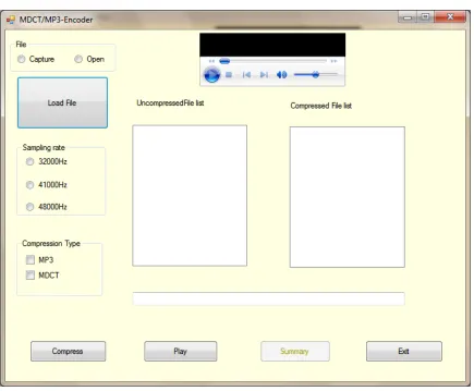
4.1 The Interface

The different project modules that formed the various project development steps were all integrated in the Interface shown in Figure 4.1. These steps included capturing of raw uncompressed waveform samples, to MP3 encoding to the final MDCT Hybrid filter bank compression. Figure 4.1 shows a picture of the front panel of the MDCT encoder.

Figure 4.1: The MDCT project Front panel.

(57)

46 4.1.1 File Open/Capture

The file to be compressed is either some already recorded audio file in the hard disk by which case the “Open” Radio button at the top left corner of the interface is checked, or a file which is directly captured and sampled at a rate chosen from the three sampling rates 32000Hz, 41000Hz or 48000Hz as grouped together in figure 4.1. The Capture Radio button initiates the recording of a new audio from a sound recording device, which is then saved before compressing.

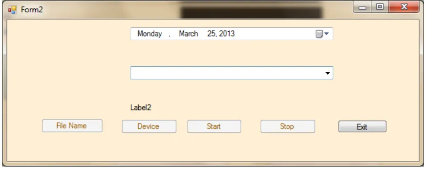
The window in Figure 4.2 is the recording interface. It contains buttons for Naming the raw file (File Name button). The “Device” button creates a list of the available recording devices. Once the recording device is selected by clicking the drop down button from the combobox below the date, then the file is given a name and stored at a chosen location accessed by clicking the “File Name” command. The recording begins when the “Start” command is clicked, and stopped with the “Stop” command. The application can be closed using the “Exit” button.

(58)

47 4.1.2 Sampling Rate

There are generally three sampling rates used in the MP3 encoding, which are 32,000Hz, 41,000Hz and 48,000Hz. The interface in figure 4.1 provides the option of choosing any of these rates by checking the respective Radio button.

4.1.3 Compression Type

Figure 4.1 provides options in form of checkboxes through which the audio file may be compressed by use of either the Standard MPEG or the MDCT laced MP3, or both. Checkboxes have been preferred over option buttons so that it makes it easy in the situation where the two compression methods need to be compared.

4.1.4 File Manipulation

(59)

48 Figure 4.3: File compression summary window.

4.1.5 Miscellaneous

The Windows Media Player component at the top of figure 4.1 makes it easy to play, pause, rewind or stop an audio file while it is being played. The compressed files are displayed on the compressed file list and the uncompressed ones on the respective file list box.

4.2 Quantitative Analysis

(60)

49

represent the RIFF header that must proceed any data to be captured from input sources. Each signal therefore has an extra 44 bits that represent the header.

Table 4.1: Compression percentages for audio signals at a sampling rate of 32000Hz

AUDIO FILE UNCOMPRESSED

FILE SIZE ON DISK (BITS)

COMPRESSED FILE SIZE ON DISK (BITS)

COMPRESSION PERCENTAGE

AUDIO1_32.WAV 6560044 616464 90.60 %

AUDIO2_32.WAV 1376044 130464 90.52 %

AUDIO3_32.WAV 1472044 139104 90.55 %

AUDIO4_32.WAV 1616044 152928 90.54 %

AUDIO5_32.WAV 4160044 391392 90.59 %

AUDIO6_32.WAV 1568044 148176 90.55 %

AUDIO7_32.WAV 1616044 152928 90.54 %

AUDIO8_32.WAV 1456044 137808 90.54 %

AUDIO1_41.WAV 1886044 185154 90.18 %

AUDIO2_41.WAV 1681044 165510 90.15 %

AUDIO3_41.WAV 1332544 131656 90.12 %

(61)

50

AUDIO5_41.WAV 1845044 181393 90.17 %

AUDIO6_41.WAV 2070544 203127 90.19 %

AUDIO7_41.WAV 1168544 115355 90.13 %

AUDIO8_41.WAV 2562544 251192 90.20 %

AUDIO9_41.WAV 1988544 195186 90.18 %

AUDIO10_41.WAV 2706044 265403 90.19 %

AUDIO1_48.WAV 2544044 213120 91.62 %

AUDIO2_48.WAV 1704044 143232 91.59 %

AUDIO3_48.WAV 2880044 241152 91.63 %

AUDIO4_48.WAV 1824044 153216 91.63 %

AUDIO5_48.WAV 2304044 193152 91.62 %

AUDIO6_48.WAV 2472044 206976 91.63 %

AUDIO7_48.WAV 1968044 165120 91.61 %

AUDIO8_48.WAV 5976044 499200 91.65 %

AUDIO9_48.WAV 2256044 189312 91.61 %

(62)

51

From the three table results, it can be seen that there was just over 90% reduction in the compression when the MDCT filtering was applied. There 41 KHz audio compression in table 4.2 shows a more improved compression than both 32 KHz and 48 KHz. The reason for this is due to the fact that during the sampling process, there are rounding offs involved when dividing the samples of 41,000 into groups of 16 bits.

The other two sampling rates perfectly fit the 16 bit divisions. It is also observed that the higher the sampling rate the smaller the percentage improvement in the compression. This can be attributed to the fact that the more samples taken during the sampling process, the closer we are able to approximate our signals to the real analogue values.

The high perccentage compression is very significant in reducing huge files to small sizes that can easily be transmitted through digital media. Large uncompressed audio files of sizes amounting to Gigabytes now get sized down to tiny chunks of Kilobytes.

Table 4.4: Compression ratios for MP1, MP2 and MP3 compression techniques for audio signals at a sampling rate of 44100Hz (David and Price, 2012).

MPEG LAYER1 MPEG LAYER2 MPEG LAYER3

(MP3) Raw Data Rate

(stereo at 44.1K samples per second

(63)

52 Compressed Data

Rate

384 kbps 192 kbps 128 kbps

Typical Compression

4:1 8:1 12:1

Table 4.4 shows the different types of audio compression used in MPEG systems and the relative amount of compression that they can provide (David and Price, 2012). This table uses a 2 channel stereo signal that is sampled at 44.1k samples per second, 16 bits per sample as a reference. The MPEG layer 1 coder can compress this signal to approximately 384 kbps (4:1 compression). The MPEG layer 2 coder can compress the signal to 192 kbps (8:1 compression). The MP3 coder can compress the signal to 128 kbps (12:1 compression). Comparred to the results obtained using the decoder developed in this project as shown in table 4.2; the compression ratios for MP3 sampled at 44.1 KHZ given as 12:1 from the cited material, closely match.

4.3 Qualitative Analysis

4.3.1 Subjective Testing

(64)

53

Table 4.5: Listening Tests Grading Scale based on ITU-R BS.1284 standard ranging from 1.0 to 5.0 (Sporer, 1997).

QUALITY IMPAREMENT 5.0 Excellent 5 Imperceptible

4.0 Good 4 Perceptible but not annoying 3.0 Fair 3 Slightly annoying

2.0 Poor 2 Annoying

1.0 Bad 1 Very annoying

One of the objectives of this project was to establish whether the MDCT encoding would produce a better compression without compromising on signal quality. This was achieved through the following method:

1. Generating an uncompressed wave audio file, called “*.wav”. Where * is the name of the input file.

2. Compressing the input file into an MP3 using the MDCT hybrid filter. 3. Playing back the audio file using the Windows Media player component.

(65)

54

options shown in table 4.6 after listening to both the raw uncompressed signal and the compressed MDCT signal.

Table 4.6: Listener satisfaction survey questionnaire.

Range in Percentage Listener’s Choice

96 – 100 20

91 – 95 None

86 – 90 None

80 – 85 None

Less than 80 None

All the volunteers clicked the 96% to 100% option, confirming that the quality of the compressed signal closely matched that of the original uncompressed one. In comparison, these results mapped to the ITU-R BS.1284 test grading system which would be viewed as table 4.7 below shows that the audio quality of the compressed audio can be concluded as excellent.

Table 4.7: Table showing comparrisons between the test results of the study, with the ITU-R BS.1284 grading system.

Percentage values ITU-R BS.1284 Mapping

96 – 100 5.0

90 – 95 4.0

81 – 89 3.0

Less than 80 2.0

Less than 80 1.0

(66)

55

Considering the Sampling rates available for audio sampling, there was a tradeoff between Audio Quality vs. Data Rate. The higher the bit rate, the higher the quality of the audio signal. However, Sampling rates do not affect file size as much as bit rates do. Bit rates of 128kbps were used in this project.

Furthermore, Audio1_32.wav sample audio file recorded as a raw uncompressed PCM was played back using the standard Media player packaged with Windows operating system, and the waveform in figure 4.4 was observed. It represents sound pressure observed against the time the music takes to play.

(67)

56 Figure 4.4: Audio1_32.wav waveform.

Figure 4.5: Audio1_32.mp3 waveform.

(68)

57 when listened to during playback.

Both figure 4.4 and figure 4.5 are screen captures captured after 20 seconds of playback time for both the uncompressed and the compressed audio file. The length of time it takes to playback both files is the same.

The similarities of the waveforms in figure 4.4 and figure 4.5 can better appreciated through the combination area graph in figure 4.6. The section Labeled A represents the waveform of figure 4.4, while the area labeled B represents the waveform in figure 4.5.

(69)

58

It should be noted that the similarities observed is a confirmation that despite the loss of uneccesary samples in the compressed audio signal, the fidelity of the final file is quite close to the CD quality PCM audio file.

4.2.2 Objective Testing

The subjective testing technique is generally time consuming and expensive. The objective testing technique uses a cognitive model in PEAQ which imitates the cognitive processing system of the human brain. The human brain cognitive process is used to compute a quality score for audio signals. The cognitive model processes in PEAQ use the parameters that are produced by the psychoacoustic human ear models to generate output values known as Model Output Variables (MOVs). Following the production of the MOVs, the values are mapped to a single Objective Difference Grade (ODG) score. There are 11 MOVs associated with the Basic Version and 5 MOVs associated wih the Advanced Version. These MOV values eventually enter a Multi-Layer Perceptron Neural Network (MLPNN). The training of the neural network software produces the ODG scores. The training itself requires that a large collection of human subjective data values obtained from listening tests (Campbell, 2009).

(70)

59

output variable obtained from the objective measurement method that use used in PEAQ and it corresponds to a Subjective Difference Grade (SDG) in the subjective testing method.

The SDG value obtained from the analysis of the results from the subjective listening test is defined as:

SDG = Grade Signal under test – Grade Reference signal (Salovarda, 2004).

Table 4.8 gives the relationship between the subjective gradings of Table 4.7 with the SDGs.

Table 4.8: SDG description

Impairment Grade SDG

Imperceptible 5.00 0.00

Perceptible but not annoying 4.00 -1.00

Slightly annoying 3.00 -2.00

Annoying 2.00 -3.00

Very annoying 1.00 -4.00

(71)

60

was evaluated using PEAQ algorithm. Table 4.9 Shows the OGV values obtained from the evaluation.

Table 4.9: Objective Difference Grade (ODG) scores for ten audio samples sampled at 48 kHz, 16-bit PCM

Reference WAV sample Degraded MP3 sample ODG values AUDIO1_48.WAV AUDIO1_48.MP3 -0.616 AUDIO2_48.WAV AUDIO2_48.MP3 -0.540 AUDIO3_48.WAV AUDIO3_48.MP3 -1.792 AUDIO4_48.WAV AUDIO4_48.MP3 -0.407 AUDIO5_48.WAV AUDIO5_48.MP3 -1.102 AUDIO6_48.WAV AUDIO6_48.MP3 -0.571 AUDIO7_48.WAV AUDIO7_48.MP3 -1.871 AUDIO8_48.WAV AUDIO8_48.MP3 -0.886 AUDIO9_48.WAV AUDIO9_48.MP3 -0.844 AUDIO10_48.WAV AUDIO10_48.MP3 -1.771

(72)

61 4.2.3 Objective Tests results from other works

Table 4.91 shows the results of tests previously taken from various codecs by the use of the PEAQ measurement software as recommended by the ITU-R BS.1387. These codecs are the standard MP2 and MP3 Lame (also named as MPEG 1 layer 2 and layer 3 respectively, based on ISO/IEC 11172/3, 1992. ISO/IEC stands for International Standards Organization/International Electrotechnical Commission), Advanced Audio Coding (AAC), according to ISO/IEC 13818/3, 1994.) And OGG Vorbis from Xiph.org, and is different from MPEG 1 and 2 standards (Salovarda et al, 2004).

All the codecs aforementioned use perceptual coding or psychoacoustic methods to perform lossy compression. The differences among them is therefore in their algorithms and and on how complex they are. They do not behave in a similar manner as can be observed from the results of the measurements (Salovarda et al, 2004).

Table 4.91: ODG values and file size for four codecs on most common bit rates (Salovarda et al, 2004).

BIT RATES CODEC ODG FILE SIZE

32 kbps

MP2 -3.85 56 KB

MP3 -3.67 56 KB

AAC

OGG 64 kbps

(73)

62

MP3 -3.46 112 KB

AAC -3.36 111 KB

OGG -3.24 113 KB

128 kbps

MP2 -2.36 222 KB

MP3 -1.08 223 KB

AAC -1.09 222 KB

OGG -0.34 221 KB

160 kbps

MP2

MP3 -0.47 276 KB

AAC -0.41 278 KB

OGG -0.20 271 KB

192 kbps

MP2 -0.59 332 KB

MP3 -0.16 334 KB

AAC -0.20 333 KB

OGG -0.09 326 KB

256 kbps

(74)

63

MP3 -0.01 445 KB

AAC -0.12 429 KB

OGG 0.02 460 KB

320 kbps/

350kbps -ogg MP2

MP3 0.04 556 KB

AAC -0.02 535 KB

OGG 0.07 632 KB

(75)

64

CHAPTER FIVE

CONCLUSIONS AND RECOMMENDATIONS

5.1 Conclusions

In this study, it has been demonstrated that MDCT encoding process provides a further reduction in the number of bits that can be used to represent an audio signal without affecting the listening experience by listeners. The PEAQ encoding technique employs the technique by observing and analyzing the human ear and the auditory system, all the while trying to refine the psychoacoustic model, and at the same time allowing the model to mathematically determine what information can be discarded from the data. The final result is an encoding technique that allows for very high compression ratios compared to its lossless counterparts.Both subjective and objective evaluations of the compressed audio files in this study were performed using Listening tests and using Perceptual Evaluation of Audio Quality (PEAQ) algorithm respectively.

(76)

65 5.2 Recommendation for future work

(77)

66

REFERENCES

Arjona, M. Ramírez, M. (2008). Technology and standards for low-bit-rate coding methods. In The Handbook of Computer Networks, 2: 447–467.

Brandenburg, K. (1987). Evaluation of quality for audio encoding at low bit rates. Contribution to the 82nd AES Convention, preprint 2433. London, United Kingdom. 100 Rec. ITU-R BS.1387-1.

Brandenburg, K. and Stoll G. (2009). ISO-MPEG-1 Audio: A Genereic Standard for Coding of High Quality Digital Audio. Journal of the Audio Engineering Society, 10: 780-792.

Bosi, M. (1997). ISO/IEC MPEG-2 Advanved Audio Coding, Journal of the Audio Engineering Society, 10: 789-813.

Campbell,D, Edward, J. and Martin, G. (2009). National University of Ireland, Galway. Audio Quality Assessment Techniques – A Review, and Recent Developments Chiariglione, L. (2009). Riding the Media Bits. MPEG's first Steps.

Davis, P. (2005). A Tutorial on MPEG/Audio Compression. IEEE Multimedia systems and applications, 2(2): 60-74.

David, L. and Price, H. (2012). MPEG codec comparrison. In Introduction to MPEG (p. 19). Althos.

Rao, K. and Yip, P. (1990), Discrete Cosine Transform. In Wikipedia. Retrieved May 15, 2012 from http://en.wikipedia.org/wiki/Discrete_cosine_transform

Dobson, K., Yang, J., Smart, K., and Guo, K. (1997). High Quality Low Complexity Scalable Wavelet Audio Coding, in Proceedings of IEEE International Conference on Acoustics, Speech and Signal Processing (ICASSP), 97: 327-330 Jacaba J. (2001). Department of Mathematics College of Science, The University of the Philippines Diliman, Quezon City. Audio compression using modified discrete cosine transform.

Junyong, Y., Ulrich, R., Miska, M., Hannuksela, B., Moncef, G. and Andrew, P. (2010). Perceptual-based quality assessment for audio–visual services: A survey

Compressionion of pulse code modulation signal using type IV discrete cosine transform based on the mp3 model

USING TYPE IV DISCRETE COSINE TRANSFORM BASED ON

THE MP3 MODEL.

BY:

TABLE OF CONTENTS