An Equivalent Method of Position Error Caused by The Array
Antenna Deformation
Xiu Tiao Ye, Wen Tao Li*, and Wen Hao Du
Abstract—The deformation of antenna array due to external factors results in a significant degradation in the performance of the array direction of arrival (DOA) estimation. To solve this problem, an equivalent method based on the estimation of signal parameters by rotational invariance technique (ESPRIT) in single signal source for the array position errors is proposed in this paper. This method is mainly for the low-order deformation of the array and is based on the equivalent value of the position error. The DOA estimation of ESPRIT algorithm for single signal source was corrected. The simulation results show that the position error equivalent method can effectively equalize the position error caused by the vibration deformation of the array. When the equivalent position error is known, the orientation of the single signal source can be effectively corrected.
1. INTRODUCTION
The direction of arrival (DOA) estimation is an important part of array signal processing. Common DOA estimation methods are multiple signal classification (MUSIC), Capon, and estimation of signal parameters by rotational invariance technique (ESPRIT) algorithms. However, when the array antenna is deformed by an external force in the actual application, the offset error of the array element will be produced [1–3]. The array offset error will result in azimuth-dependent array gain and phase errors, which could lead to the performance degradation of the array antenna DOA estimation algorithm. Therefore, it is necessary to calibrate the gain and phase errors to overcome this problem.
At present, the calibration technology for gain and phase errors of the array is divided into two categories: self-calibration method [4–8] and active calibration method [9–11]. The self-calibration method is used to estimate the error through the combination of array error parameters and azimuth estimation. In [4], Friedlander and Weiss proposed a subspace-based self-calibration algorithm in which the DOA estimated angle was obtained by searching for two-dimensional spectral peak. In [5], a correction method of the array element position error with near-field correction source was proposed based on the weighted signal subspace fitting technique.
The active calibration algorithm needs calibrated signal sources to calculate the gain and phase errors. In [9], a method of position error correction based on maximum likelihood criterion, with known correction source waveform, was proposed. In [11], an active method based on the conventional subspace fitting was proposed to estimate the array shape.
The ESPRIT algorithm was first proposed by Roy et al. in 1986 [12]. In the ESPRIT algorithm, the array is divided into two identical subarrays [13]. The rotation invariance of the subarray generated by the displacement invariance of the subarray is used to solve the direction of the signal according to the rotation phase between the subfields of the subarray. Compared with other high-resolution DOA estimation algorithms, this algorithm does not need angle search, and the estimation result can be directly calculated [14–16].
Received 8 January 2018, Accepted 8 March 2018, Scheduled 20 March 2018 * Corresponding author: Wen Tao Li ([email protected]).
In this paper, an equivalent length model is proposed to solve the position error of the array under the single signal source. Based on the equivalent length, the DOA estimation can be corrected by improving the traditional ESPRIT algorithm. When the direction of a single signal source is known, the equivalent length can be calculated. Compared to the traditional active correction algorithm, which needs to calculate the position error of each element, the proposed method only needs to calculate the equivalent length, which can effectively reduce the computational complexity.
2. VIBRATION AND SIGNAL MODELS
2.1. Array Deformation Model
It is presumed that the array antenna carrier is a rigid substrate. When vibration or static deformation occurs in the array, the substrate is generally shown as modal changing. The low-order deformation model of the rigid substrate can be described by:
z1(x) = h 3l40
x4−4l0x3+ 6l20x2 (1)
whereh is the maximum displacement of the substrate tip in the vertical direction,l0 the length of the substrate, and z1(x) the displacement of the substrate at thexcoordinate. The deformation model can be derived from the vibration model proposed in [17].
The substrate length was assumed equal to 1 (l0 = 1). Fig. 1 illustrates the deformation curves of the substrate when the maximum displacement of the substrate tip takes different values calculated in Eq. (1). In addition, another three curves were also employed in the simulations: z2= 1.56h(x−0.2)2, z3= 3h(x−0.3)3,z4 = 7.7h(x−0.4)4.
Figure 1. Array antenna deformation curve.
2.2. Signal Model
Presuming that the array antenna is a uniform linear array (ULA), the number of elements will beM+1; there areN signal sources in the unknown space, and the direction of the signal source isθ1, θ2, . . . θN.
The array elements are distributed on the substrate. The formerM elements are composed of subarray X, and the latter M elements are composed of subarray Y. The interval between the two subarrays is half wavelength. The received data of the two subarrays are respectively:
x(t) = As(t) +nx(t) (2)
where x(t)= [x1(t) x2(t). . . xM(t)]T and y(t)= [y1(t) y2(t). . . yM(t)]T represent the received data of
the respective elements in the subarrays X and Y; s(t)= [s1(t) s2(t). . . sN(t)]T is the signal data
of the kth signal source; A = [a(θ1) a(θ2) . . .a(θN)] is the response matrix of subarray X, wherein a(θk)= [a1(θk)a2(θk) . . . aM−1(θk)]T, andk= 1,2, . . . N is the corresponding angle θk of the subarray
X. The matrixΦ=diag{ejωkΔxsinθ1 ejωkΔxsinθ2 . . . ejωkΔxsinθK}is a diagonal matrix, which represents the spatial delay caused by the spacing of theY subarrays relative to theXsubgroup at different incident angles.
At the receiving end, K snapshots data were sampled at time points t=t1, t2, . . . tK. Hence, the
received data x(t) and y(t) became the M×N dimensional data matrix, and Eqs. (2) and (3) can be expressed as:
X = AS+Nx (4)
Y = ΦAS+Ny (5)
where X= [x(1) x(2) . . . x(K)] and Y= [y(1) y(2) . . . y(K)] represents the data matrix consisting of K snapshots of subarrays X and Y, respectively; S= [s(1) s(2) . . . s(K)] represents the data matrix containing K snapshots emitted by different sources, and Nx = [nx(1) nx(2) . . . nx(K)] and Ny = [ny(2) ny(2) . . . ny(K)] represents the noise matrix containing K snapshots.
The received data matrix Zof the entire array is
Z=
X Y
=AS¯ +Nz (6)
where A¯=[ A
AΦ ] is the response matrix of the array, andNz = [ Nx
Ny ] represents the noise matrix of
the array.
The covariance matrix of the array is
Rzz =EZ(t)Z(t)H=AR¯ ssA¯ +σ2I (7) whereRss is the covariance matrix of the received signal data, and σ2 is the noise variance.
3. FORMULATION OF DESIGN PROBLEM
There are many ways to implement the ESPRIT algorithm. Here, we take the least squares (LS) as an example to introduce the implementation process of ESPRIT algorithm. The procedure for the LS-ESPRIT algorithm is:
a) According to Eq. (7), the covariance matrixRˆzz can be calculated from the array receiving matrix
Z;
b) The matrix Ais decomposed by eigenvalues, and it can be obtained through:
ˆ
RzzE= ΛE (8)
where Λ = diag{λ1 λ2. . . λM+1} satisfies the condition of λ1 ≥ . . . λN > λN+1 = . . . = λM+1;
E= [e1 e2. . .eM+1] and ei represent the eigenvector corresponding to the eigenvalueλi;
c) These eigenvectors corresponding to the N largest eigenvalues in matrix Rˆzz can be constructed as the signal subspace of the array. Hence, the signal subspace can be divided intoEx andEy;
d) The matrix D can be calculated as follows:
D=E+xEy (9)
whereE+x is the pseudo inverse ofEx. Then,D is decomposed by eigenvalues, and the eigenvalue
˜
e) The arguments are obtained from the eigenvalue ˜λi, i = 1,2. . . N, and the DOA estimation of
different direction source could be obtained as follows:
θi= arcsin
angle(λi)
2πd i= 1,2. . . N (10)
where angle(•) represents the operation of obtaining the argument, andd represents the ratio of the element spacing to the wavelength.
As the array receives data from a single signal source whose direction isθ0, the received data will be:
x(t) = ax(θ0)s(t) +nx(t) (11)
y(t) = Fax(θ0)ejϕs(t) +ny(t) (12)
Here, ϕ = 2πdsin(θ0), and the steering vector ax(θ0) represents the post-deformed subarray X. The matrixF is
F= diag
ej2πcos(θ0)Δx1 ej2πcos(θ0)Δx2 . . . ej2πcos(θ0)ΔxM (13)
where the matrix Frepresents the phase error caused by position errors Δx1Δx2 . . . ΔxM.
According to the subspace theory, the response matrixAof the array satisfies the relationship with the signal subspaceE, wherein:
E=AT (14)
As the array receives only one signal source, the response matrixAdegrades into the steering vector a:
a=
ej2π[sin(θ1)0d+cos(θ0)x1] . . . ej2π[sin(θ1)(M−1)d+cos(θ0)xM] (15)
where, x1 x2 . . . xM are the position errors of the subarrayX; the full-rank matrix Tis degraded to a
constant t, and the signal subspace matrix E is degraded to a (M + 1) dimension vectore. Then, the subspaces corresponding to the two subarrays satisfy:
e= ex ey = at
Faejϕt
(16)
When Eq. (15) is taken into matrix D in step (d), the matrix D is degraded to a constant g, in which:
g=e+xey =eHx ex−1eHxey =tHaHat−1tHaHFaejϕt= e
jϕ
M a
HFa (17)
If Eqs. (13) and (14) are brought into Eq. (17), we can obtain:
g= e
jϕ
M a
HFa= ejϕ
M
ej2πcos(θ0)Δx1 +ej2πcos(θ0)Δx2. . .+ej2πcos(θ0)ΔxM (18)
Here, we assume that Eq. (17) can be approximated through an equivalent length ˜l:
ejϕ M
ej2πcos(θ0)Δx1 +ej2πcos(θ0)Δx2. . .+ej2πcos(θ0)ΔxM≈ejϕej2πcos(θ0)˜l (19)
where ˜l is the equivalent length of the position error, and Eq. (19) implies that both sides are approximately equal at any angle θ0.
After the calculation of the argument of both sides in Eq. (19), it is determined to be:
sin(Δx1B(θ0)) + sin(Δx2B(θ0)). . .+ sin(ΔxM−1B(θ0))
cos(Δx1B(θ0)) + cos(Δx2B(θ0)). . .+ cos(ΔxM−1B(θ0))
≈tan ˜ lB(θ0) (20)
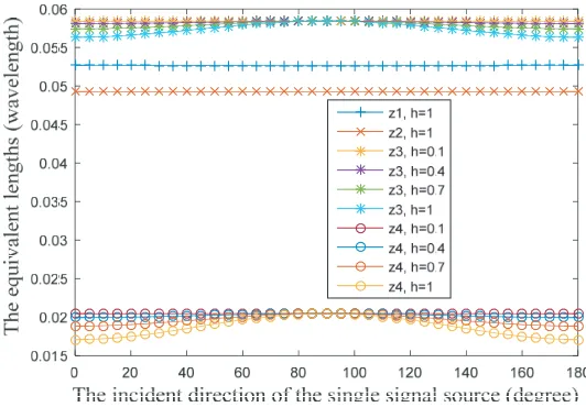
Figure 2. The equivalent lengths of the curves correspond to different angles.
4. NUMERICAL RESULTS
Using the curves described in Section 2 as the deformation data, the number of elements (M+ 1) is 20. In [0, 1], 20 coordinate points are evenly sampled as the element position. In the [0, 180◦] range, θ is taken as a different value, and the corresponding equivalent length can be calculated as shown in Fig. 2. It can be observed in Fig. 2 that if the array produces deformation, such as z1, z2 curves, the equivalent lengths corresponding to each angles are similar. However, if the array produces deformation like z3,z4 curves, the equivalent lengths corresponding to different angles are not the same. Therefore, the greater the degree of deformation is, the greater the difference will be. By taking into account the actual situation of array deformation, it can be assumed that the equivalent length is effective as the array is deformed and that the equivalent length will be the same for each angle.
Assuming that the antenna array is a ULA, the number of elements (M + 1) is 20; the spacing of the array elements is half a wavelength; the signal-to-noise ratio (SNR) is 20 dB in the second example. If the arrival of the single signal source θ0 is 10◦, then the corresponding equivalent length can be calculated, using gin Eq. (18), as:
˜
l= angle(g)−2πsin(θ0)d 2πcos(θ0)
(21)
Furthermore, the direction of other signal sources can be corrected with the equivalent length. The steps in using equivalent length to correct other directions of the single signal sources are similar to that of the conventional LS-ESPRIT algorithm, except for step e), where Eq. (10) becomes:
θx= arcsin
angle(λx)/(2π)
˜ l2+d2
−arcsin
˜ l
˜l2+d2
(22)
It is assumed that the angles from 1◦ to 60◦, with 1◦ step size, are used as the incident directions of different single signal sources. Thus, 60 independent experiments are conducted for each deformation state of array.
The DOA estimation root mean square error (RMSE) is defined as:
RMSE =
L
i=1
(¯θi−θi)2L (23)
Figure 3. The DOA estimation RMSE for different deformed arrays.
Figure 4. The DOAs estimation corrected and uncorrected by equivalent length.
The DOA estimation RMSE for different single signals can be obtained under the four curves, as shown in Fig. 3. It can be seen from Fig. 3 that the correction algorithm based on the equivalent length can effectively correct the DOA estimation angle under the single signal source. Moreover, it can also be observed in Fig. 3 that with deepened degree of deformation, the equivalent lengths of z3 and z4 curves corresponding to different angles become inconsistent but are still able to effectively complete the correction.
In the third example, the array is chosen in the same manner as in the second example. Assuming that there are N = 3 signal sources in the unknown space, the SNRs of each signal sources are 20 dB. The signal source, with the incident direction θ1 = 10◦, is known as the correction signal source. Other signal sources have directions of 40◦ and 50◦.
In step (e), the equivalent length is first calculated using the eigenvalue λ1 corresponding to the 10◦ signal, wherein:
˜
l= angle(λ1)−2πsin(θ1)d
Then, the DOAs estimation for the other directions can be corrected using the equivalent length ˜l, in which:
θi = arcsin
angle(λ i)/(2π)
˜ l2+d2
−arcsin
˜ l
˜ l2+d2
i= 2,3. . . N (25)
The curve z1 is used as the deformation model of the array, and the tip h of the substrate is gradually changed from 0 to 0.5λ. The DOAs estimation corrected by equivalent length are calculated at different deformations and compared with the traditional ESPRIT algorithm (uncorrected) estimates, shown in Fig. 4. It can be seen from Fig. 4 that although varying degrees of deformation occur in the array, the algorithm proposed in this paper is still effective and able to maintain high precision and stability.
5. CONCLUSIONS
An equivalent length model of position error based on the ESPRIT algorithm and caused by low-order deformation of the array under single signal source is proposed in this paper. The equivalent length can be used to calibrate the DOA estimation error of the single signal source. Moreover, simulation results show that the proposed approach is also effective when multiple single sources are considered. Compared with the traditional active correction algorithm, which is necessary for calculating the position error of each element, the proposed method only needs to calculate the equivalent length and reduce computational complexity.
ACKNOWLEDGMENT
This work was supported in part by the National Natural Science Foundation of China (No. 61571356), in part by the Fundamental Research Funds for the Central Universities (No. JB180203), in part by ZTE Technologies, and in part by the Shaanxi Natural Science Foundation.
REFERENCES
1. Arnold, E. J., Y. B. Yan, R. D. Hale, F. Rodriguez-Morales, P. Gogineni, J. Li, and M. Ewing, “Effects of vibration on a wing-mounted ice-sounding antenna array,” IEEE Antennas Propag.
Mag., Vol. 56, No. 6, 41–52, 2014.
2. Du, Q. and P. Du, “Computation of fluctuating wind pressure and wind loads on phased-array antennas,”IEEE Antennas Propag. Mag., Vol. 54, No. 1, 66–75, 2012.
3. Wang, C., M. Kang, W. Wang, B. Duan, L. Lin, and L. Ping, “On the performance of array antennas with mechanical distortion errors considering element numbers,”Int. J. Electron., Vol. 104, No. 3, 462–484, 2017.
4. Friedlander, B. and A. J. Weiss, “Eigenstructure methods for direction finding with sensor gain and phase uncertainties,” Circuits Syst. Signal Process., Vol. 9, 272–300, 1990.
5. Wijnholds, S. J. and A. J. V. D. Veen, “Multisource self-calibration for sensor arrays,”IEEE Trans.
Signal Process., Vol. 57, No. 9, 3512–3522, 2009.
6. Weiss, A. J. and B. Friedlander, “Array shape calibration using sources in unknown locations — A maximum likelihood approach,” IEEE Trans. Acoust. Speech Signal Process., Vol. 37, No. 12, 1958–1966, 1989.
7. Flanagan, B. P. and K. L. Bell, “Array self-calibration with large sensor position errors,” IEEE
Trans. Signal Process., Vol. 81, No. 10, 2201–2214, Oct. 2001.
8. Lanagan, B. P. and K. L. Bell, “Array self-calibration with large sensor position errors,” Signal
Process., Vol. 81, No. 11, 2201–2214, 2001.
10. Ng, B. C. and A. Nehorai, “Active array sensor location calibration,” IEEE Proc. ICASSP, Vol. 4, 21–24, 1993.
11. Park, H. Y., C. Lee, D. H. Youn, and H. G. Kang, “Generalization of the subspace-based array shape estimations,” IEEE J. Ocean. Eng., Vol. 29, No. 3, 847–856, 2004.
12. Roy, R., A. Paulraj, and T. Kailath, “ESPRIT-A subspace rotation approach to estimation of parameters of cisoids in noise,” IEEE Trans. Acoust., Speech. Signal Processing, Vol. 34, 1340– 1342, Oct. 1986.
13. Qian, C., L. Huang, and H. C. So, “Computationally efficient ESPRIT algorithm for direction-of-arrival estimation based on Nystr¨om method,”Signal Process., Vol. 94, No. 1, 74–80, 2014. 14. Kim, S., D. Oh, and J. Lee, “Joint DFT-ESPRIT estimation for TOA and DOA in vehicle FMCW
radars,”IEEE Antennas Wirel. Propag. Lett., Vol. 14, 1710–1713, 2015.
15. Cui, K., W. Wu, J. Huang, X. Chen, and N. Yuan, “2-D DOA estimation of LFM signals for UCA based on time-frequency multiple invariance ESPRIT,”Progress In Electromagnetics Research M, Vol. 53, 153–165, 2017.
16. Li, J., M. Jin, Y. Zheng, G. Liao, and L. Lv, “Transmit and receive array gain-phase error estimation in bistatic MIMO radar,” IEEE Antennas Wirel. Propag. Lett., Vol. 14, 25–32, 2015.
17. Schippers, H., J. H. van Tongeren, and G. Vos, “Development of smart antennas on vibrating structures of aerospace platforms of conformal antennas on aircraft structures,”Proc. NATO AVT