Scholarship@Western
Scholarship@Western
Electronic Thesis and Dissertation Repository
9-13-2016 12:00 AM
Formation and Past Evolution of the Meteoroid Complex of Comet
Formation and Past Evolution of the Meteoroid Complex of Comet
96P/Machholz
96P/Machholz
Abedin Yusein Abedin
The Univerisity of Western Ontario Supervisor
Prof. Paul A. Wiegert
The University of Western Ontario Joint Supervisor Prof. Peter G. Brown
The University of Western Ontario Graduate Program in Astronomy
A thesis submitted in partial fulfillment of the requirements for the degree in Doctor of Philosophy
© Abedin Yusein Abedin 2016
Follow this and additional works at: https://ir.lib.uwo.ca/etd
Part of the The Sun and the Solar System Commons
Recommended Citation Recommended Citation
Abedin, Abedin Yusein, "Formation and Past Evolution of the Meteoroid Complex of Comet 96P/ Machholz" (2016). Electronic Thesis and Dissertation Repository. 4148.
https://ir.lib.uwo.ca/etd/4148
This Dissertation/Thesis is brought to you for free and open access by Scholarship@Western. It has been accepted for inclusion in Electronic Thesis and Dissertation Repository by an authorized administrator of
Abstract
The past dynamical evolution of the meteoroid streams associated with comet 96P/Machholz is investigated. The goal is to obtain a coherent picture of the past capture of this large comet into a short period orbit, and its subsequent breakup hierarchy. In particular, the aim is to constrain the earliest epoch that this large first precursor started to supply meteoroids into the interplanetary space. The fragments and meteoroid streams of that past cometary decay con-stitute a wide multiplex of interplanetary bodies, knows as the 96P/Machholz complex. The largest presently surviving fragment is comet 96P/Machholz, followed by a large amount of debris including the Marsden and Kracht group of sungrazing comets, as well as at least one object of asteroidal appearance e.g., asteroid 2003 EH1.
It has been recognized that comet 96P/Machholz can give rise to eight different meteor showers within one Kozai secular cycle. These are the Quadrantids, daytime Arietids, Southern and Northernδ-Aquariids,κ-Velids,θ-Carinids,α-Cetids and the Ursids. The first four showers are strong and well defined. The remaining four showers are weaker and less well constrained. In fact, while the activity of the Southern and Northernδ-Aquariids and κ-Velids, θ-Carinids stands well above the sporadic meteor background, the existence of theα-Cetids and the Ursids, and their association with comet 96P/Machholz is uncertain.
Recently, some of these meteor showers have been associated with the Marsden group of sunskirting comets, based on orbital similarity and past dynamical evolution. The fact that these meteoroid streams are associated with more than one parent strongly suggest a possible genetic relationship between these bodies.
Using large-scale numerical simulations, the formation and past evolution of each individ-ual meteoroid stream, associated with comet 96P/Machholz and the Marsden group of comets, is explored. Then the simulated shower characteristics are compared with observed ones as constrained by different meteor detection surveys (radar, TV, video, photographic and visual).
In the first part of this work, the formation and likely age of the Quadrantids, the strongest among the eight meteor showers, is examined. The Quadrantids are unusual with their very short duration of maximum activity (∼17 hours) superimposed over a long-lasting weaker ac-tivity. The short duration of the peak activity indicates a narrow stream which on the other hand suggest that it must be young. Using numerical simulations it is demonstrated that the core of the Quadrantids is only 200 years old and is associated with asteroid 2003 EH1, while
the broader activity is associated with comet 96P/Machholz. The possible nature of the parent, as a dormant or recently extinct comet, is emphasized.
The second part of the work focuses on the age and likely parent of the daytime Arietids meteor shower. Due to their daytime peak activity, the observational characteristics of the Arietids are mostly constrained by radar surveys. The association of the shower with comet
be the dominant parent of the stream, though they contribute to the peak of the shower. The major parent is comet 96P/Machholz and the age of the daytime Arietids is at least 10000 years. The last part of this study investigates the origin and ages of the less-well constrained showers, the Southern and Northernδ-Aquariids,κ-Velids,θ-Carinids, and the mis-associated
α-Cetids and Ursids with comet 96P/Machholz. It is demonstrated that the gross features of the observed characteristics of the first four showers can be explained by comet 96P/Machholz while the Marsden group of comets contribute a small fraction to the peak activity of these showers. Furthermore, the association of the Northernδ-Aquariids with the Marsden group of comets, as previously suggested by several authors, is not supported by this study. Instead the bulk contributor to the shower is comet 96P/Machholz, and possibly another minor parent or parents not considered in this work. Furthermore, two showers were established as potential candidates for the misidentifiedα-Cetids and Ursids. These showers are the daytimeλ-Taurids and the much weaker Decemberα-Draconids, though the last shower spatially overlaps with the November ι-Draconids, where their separation as individual showers is difficult. Lastly, the derived ages of all showers vary between 12000-20000 years, much older than previous estimates. When these shower age estimates are put into perspective, the observed character-istics of showers are consistent with a scenario of a capture of a large first precursor of the 96P complex circa 20000 BC and its subsequent fragmentation with a major break occurring around 100 AD as origin of the sunskirting comets.
Keywords: Comet 96P/Machholz, Marsden group of comets, 96P meteoroid complex, meteoroid streams, numerical simulations.
Copyright and Permissions
This thesis consists of three papers, listed in the Co-Authorship Statement, which are pub-lished, in press or submitted to theIcarusjournal.
The journal grants first authors an explicit permission to use their work as part of their Ph.D. thesis (personal communications with the journal’s support team).
This thesis dissertation is based on several published or submitted manuscripts which are listed as follows:
• Chapter 2
Age and Formation Mechanism of the Core of the Quadrantid Meteoroid Stream:
Pub-lished in Icarus, (2015), Vol. 261, pp. 100-117. Authors: Abedin, Abedin; Spurný, Pavel; Wiegert, Paul; Pokorný, Petr; Boroviˇcka, Jiˇrí; Brown, Peter:
I prepared the initial conditions for integration of the equations of motion of 8 high-precision photographic Quadrantid backwards in time. Next, I numerically integrated backwards the equations of motion of each photographic Quadrantid along with 10000 clones and the orbit of 2003 EH1, which was the presumed parent body in this work. The
aim was to identify the epoch when the distance between the orbits of the clones and the parent was minimum. I then used that epoch as meteoroid ejection onset time and propagated the orbits of the parent and synthetic meteoroid streams forward in time, until the present. I then collected a graphed the output from the simulations. The results of the simulations were interpreted with the help of Dr. Paul Wiegert, Dr. Peter Brown and Dr. Petr Pokorny. I then prepared and submitted the manuscript to the Icarus journal. Finally, I edited the manuscript in accordance with the reviewers’ comments and suggestions. At that time we figured the necessity of toolkit, designed to automate the illustration of the results of simulation for future works, whose graphic interpretation would be similar to the current work. At that point, I started developing a toolkit, which would take the results of simulations as an input and output the results in illustrative form ready to be interpreted.
Dr. Paul Wiegert contributed to this work with providing a numerical integration pack-age and numerous of advices and comments as to how the problem has to be tackled. He also actively participated in the preparation of the manuscript providing useful com-ments and suggestions as to how the text can be improved. Drs. Pavel Spurný and Jiˇrí Boroviˇcka were mainly involved in the observations, data gathering and processing of seven high-precision photographic Quadrantids. Without their effort, this work would not be possible. Dr. Petr Pokorný contributed with useful comments on this work. Dr. Peter Brown was involved in the radar detection of the meteor showers and has kindly provided observational data on five high-precision radar Quadrantids.
• Chapter 3
The age and the probable parent body of the daytime Arietid meteor shower: Submitted toIcarusand in Press, (2016). Authors: Abedin, Abedin; Wiegert, Paul; Pokorný, Petr; Brown, Peter:
In the course of preparing this work, I spent a substantial amount of work to modify my toolkit, so more complicated problems can be solved. At this stage the toolkit was already more advanced. I prepared the initial conditions for backward integrations of the equations of motion of the two presumed parent bodies, comet 96P/Machholz and comet P/1999 J6 that represented the Marsden group of comets. I numerically integrated the equations of motion backwards in time, along with 10000 clones for each parent. I used the integration package provided by Dr. Paul Wiegert. I analyzed the results from backward numerical integrations with the help of Dr. Paul Wiegert, Dr. Peter Brown and Dr. Petr Pokorny. Using the results from these simulations, we selected an appropriate meteoroid ejection onset time and forward numerical integrations of the orbits of both parents and their synthetic meteoroid streams, until the present. I prepared and ran the simulations on the large computer cluster - the Shared Hierarchical Academic Research Computing Network (SHARCNet). I streamed the results of the forward integrations through my numerical toolkit, which provided a direct comparison of the results of sim-ulations with the observed characteristics of the daytime Arietids shower. I interpreted and analyzed the results from the simulations with the help of Dr. Paul Wiegert, Dr. Peter Brown and Dr. Petr Pokorny. I then prepared and submitted the manuscript after incorporating useful suggestions and comments from Dr. Paul Wiegert, Dr. Peter Brown and Dr. Petr Pokorny. Finally, I revised and re-submitted the manuscript in accordance with the reviewers’ comments.
Dr. Paul Wiegert contributed to this work with providing a numerical integration pack-age and with many comments and suggestions as to how the problem may be solved. In addition, he spent some time to verify some of the calculations. Dr. Petr Pokorný contributed with useful comments on this work, related to the preparation and analysis of the numerical simulations. Dr. Peter Brown was involved in radar registration and data processing pertinent to the observations of the daytime Arietids. In addition, he also provided useful comments on how to improve that work.
• Chapter 4
Formation and past evolution of the showers of 96P/Machholz complex: Submitted to
At this stage, my numerical toolkit was already rather advanced. It allowed for nu-merical simulations initiation and their redistribution across multiple computing nodes. Dr. Paul Wiegert kindly provided the integration package. I prepared the set of initial conditions for backward integrations of the orbits of comet 96P/Machholz and comet P/1999 J6 that represented the Marsden group fo comets. I fed these initial conditions to my toolkit, which using the numerical integration package, ran the jobs on multiple CPUs on SHARCNet. I used again my toolkit, which took as input the raw data from simulations and output a graphical representation of the results. At that point myself, Dr. Paul Wiegert, Dr. Peter Brown and Dr. Petr Pokorny determined the initial meteoroid ejection onset epochs for forward integration of the orbits of both presumed parent bodies along with large set of particles, representing synthetic meteoroid streams of each parent. I prepared the initial conditions for the forward simulations and using my toolkit the jobs were initiated on the SHARCNet computer cluster. Once again, the raw data from the forward simulations was input by myself to my toolkit, which compared the results of the simulations directly with the observed characteristics of the resulting meteor showers of each parent body. Moreover, the toolkit provided graphical representations of the fits from the simulations, which I interpreted with help of Dr. Paul Wiegert, Dr. Peter Brown and Dr. Petr Pokorny. Finally, I prepared and submitted initial manuscript to the Icarus journal. Subsequently, I revised the initial manuscript, along with Dr. Paul Wiegert, Dr. Peter Brown and Dr. Petr Pokorny, in accordance with the reviewers’ comments and I re-submitted the final version of the manuscript.
Dr. Diego Janches is the person who has contributed to the establishment of the Southern Argentina Agile Meteor Radar (SAAMER), which is now operational in the southern hemisphere of the Earth. Dr. Janches has also actively participated in data gathering and processing of meteor showers registered by SAAMER and associated with comet 96P/Machholz. These showers are observable from the southern hemisphere only. With-out his great contribution, this work would not be possible. Dr. Paul Wiegert contributed to this work with providing a numerical integration package and with many comments and suggestions on meteoroid stream dynamics and interpretation of results from numer-ical simulations.
Dr. Petr Pokorný contributed substantially to this work by analyzing the observational characteristics of the showers obtained by CMOR and SAAMER. In addition, he has
provided useful comments on how to improve this work. Dr. Peter Brown was involved in radar registration of the some of the meteor showers that peak in the northern hemi-sphere and provided the observational data for this work. In addition, he also provided useful comments on how to improve that work. Dr. Jose Luis Hormaechea has actively participated and contributed to this work by observational data gathering of the showers that peak in the southern hemisphere.
Abstract i Copyright and Permissions iii Co-Authorship Statement iv
List of Figures xiii
List of Tables xix
List of Appendices xx
List of Abbreviations and Symbols xxi
1 Introduction 1
1.1 Small Solar System Bodies. Motivation . . . 1
1.2 Parent bodies of meteoroids . . . 5
1.2.1 Comets . . . 5
Comet reservoirs and orbital classifications . . . 7
1.2.2 Main Asteroid Belt . . . 10
Delivery of asteroids to the near-Earth space. . . 12
1.3 Formation of meteoroid streams . . . 12
1.3.1 Cometary origin . . . 12
Ejection speeds . . . 13
Evolution of comets into asteroids . . . 15
1.3.2 Asteroidal origin . . . 16
Mass loss from asteroids . . . 16
1.4 Dynamical evolution of meteoroid streams . . . 17
1.4.1 Gravitational and secular evolution . . . 17
1.4.2 Non-gravitational forces . . . 19
Solar radiation pressure . . . 19
Poynting - Robertson drag . . . 20
1.5 Meteor detections and observations . . . 22
1.5.1 Visual observations . . . 23
1.5.2 Photographic observations . . . 24
1.5.3 Video observation . . . 25
1.5.4 Radar observations . . . 25
1.6 The meteoroid complex of comet 96P/Machholz . . . 26
1.6.1 Comet 96P/Machholz . . . 26
1.6.2 96P/Machholz complex showers . . . 28
The Quadrantids . . . 28
The Daytime Arietids . . . 28
Southern and Northernδ-Aquariids . . . 29
κ-Velids,α-Cetids, Carinids and Ursids . . . 29
2 The origin of the core of the Quadrantids 40 2.1 Introduction . . . 40
2.2 Asteroid 2003 EH1and the Quadrantids meteoroid streams . . . 43
2.3 Meteoroid ejection model . . . 47
2.3.1 Cometary sublimation . . . 48
2.4 Observational Data . . . 50
2.4.1 Photographic Quadrantids . . . 50
2.4.2 Radar Quadrantids . . . 51
2.5 Numerical Simulations . . . 55
2.5.1 The “clones” . . . 55
2.5.2 Phase 1: Backward integrations . . . 56
2.5.3 Phase 2: Forward integrations . . . 58
2.6 Results . . . 59
2.6.1 Phase 1: Meteoroid release epoch . . . 59
2.6.2 Phase 1: Formation mechanism of the Quadrantid meteoroid stream . . . . 64
2.6.3 Phase 2: Meteoroid ejection . . . 68
2.7 Discussion and Conclusions . . . 80
3 The origin of the daytime Arietids 88 3.1 Introduction . . . 88
3.2 Observations . . . 91
3.3 Numerical Simulations . . . 94
3.3.1 Stage I - Backward integrations of potential stream parent bodies . . . 94
3.3.2 Parent candidate # 1: P/1999 J6 . . . 95
Meteoroid ejection modeling . . . 98
Meteoroid ejection from parent candidate #1: P/1999 J6 . . . 99
Meteoroid ejection from parent candidate # 2: 96P/Machholz . . . 101
3.4 Results . . . 106
3.4.1 Parent candidate #1: P/1999 J6 . . . 106
3.4.2 96P/Machholz . . . 110
Cases 6 and 7. . . 111
Case 5 . . . 122
Cases 8 and 9: Discrepancy between radar and optical Arietids surveys . . 127
3.5 Discussion and Conclusions . . . 133
4 Past evolutions of the 96P/Machholz showers 139 4.1 Introduction . . . 139
4.1.1 96P/Machholz complex showers . . . 141
The Quadrantids . . . 141
The Daytime Arietids . . . 142
Southern and Northernδ-Aquariids . . . 142
κ-Velids,α-Cetids, Carinids and Ursids . . . 143
4.2 Observations . . . 143
4.2.1 Parent bodies . . . 146
4.3 Numerical Simulations . . . 149
4.3.1 Solar System model and numerical integrator . . . 149
4.3.2 Meteoroid ejection . . . 150
Selecting “clones” for backward integrations . . . 151
4.3.3 Phase 1: Backward integrations of parent body candidates . . . 152
Parent candidate #1 96P/Machholz . . . 152
Parent candidate #2 P/1999 J6 . . . 153
4.3.4 Phase2: Forward integration . . . 154
Selection of “clones” for meteoroid ejection from parent candidate #1 96P/Machholz . . . 154
Selection of “clones” for meteoroid ejection from parent candidate #2: P/1999 J6 . . . 156 Orbit integration of meteoroids ejected from parent candidate #1 96P/Machholz157 Orbit integration of meteoroids ejected from parent candidate #1 P/1999 J6 157
Weighting of meteoroids by their perihelion distance at time of ejection . . 158
Weighting by meteoroid size . . . 158
4.4 Results . . . 159
4.4.1 The simulated meteor showers of parent candidate - 96P/Machholz . . . . 160
The Quadrantids (QUA) . . . 160
The Southernδ-Aquariids (SDA) . . . 165
The Northernδ-Aquariids (NDA) . . . 169
Filament 1 . . . 171
Filament 2 . . . 175
Filament 3 . . . 179
Filament 4 . . . 182
4.4.2 The simulated meteor showers of parent candidate - P/1999 J6 . . . 186
The Southernδ-Aquariids . . . 186
Filament 1 and 3 . . . 192
Filament 4 . . . 192
4.5 Discussion and Conclusions . . . 196
5 Concluding remarks 204 A Supplementary material to Chapter 4. 206 A.1 Meteor showers of comet 96P . . . 207
A.1.1 The Quadrantids (QUA) . . . 207
A.1.2 The Southernδ-Aquariids (SDA) . . . 208
A.1.3 The Northernδ-Aquariids (NDA) . . . 209
A.1.4 Filament 1 - The Decemberα-Draconids (DAD) . . . 210
A.1.5 Filament 2 - The daytimeλ-Taurids (DLT) . . . 211
A.1.6 Filament 3 - Theθ-Carinids (TCD) . . . 212
A.1.7 Filament 4 - Theκ-Velids (KVE) . . . 213
A.2 Meteor showers of comet P/1999 J6 . . . 214
A.2.1 The Southernδ-Aquariids (SDA) . . . 214
A.2.2 Filament 4 - Theκ-Velids (KVE) . . . 215
A.3 Combined activity of 96P and P/1999 J6 . . . 216
A.3.1 Southernδ-Aquariids . . . 216
A.3.2 Filament 4 - Theκ-Velids (KVE) . . . 217
B Celestial reference frames 218 B.1 Ecliptic and equatorial celestial coordinates . . . 218
D Definitions 225
Curriculum Vitae 227
List of Figures
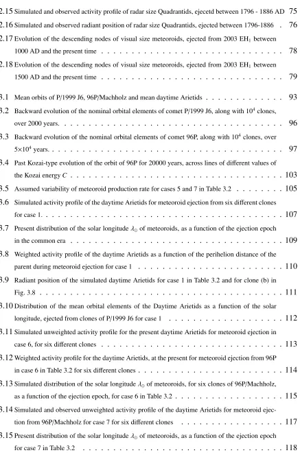
1.1 Size-mass distribution of some known objects . . . 4
1.2 Illustration of a comet nucleus . . . 6
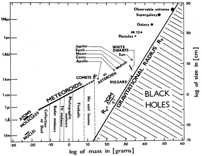
1.3 Main components of an active comet . . . 7
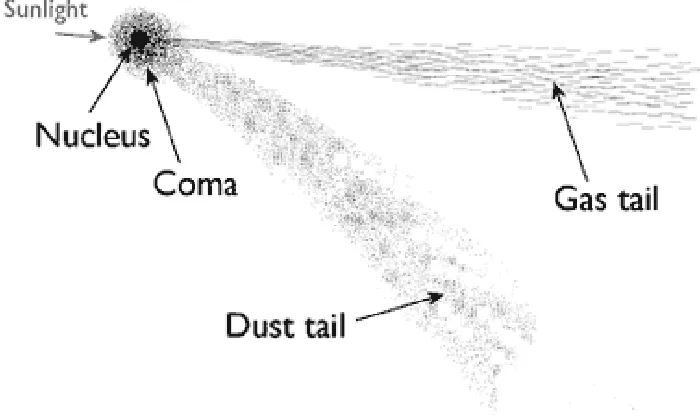
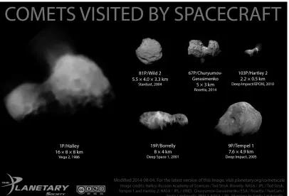
1.4 Shapes and sizes of some comets, visited by spacecrafts . . . 8
1.5 Illustration of the Edgeworth-Kuiper belt . . . 9
1.6 Illustration of the Oort cloud. . . 10
1.7 Illustration of the Main Asteroid Belt . . . 11
1.8 Illustration of the Poynting-Robertson effect . . . 21
1.9 Illustration of meteoroid encounter geometry . . . 23
2.1 Orbits of asteroid 2003 EH1and the mean Quadrantid stream . . . 45
2.2 Average visual activity profile of the Quadrantid meteor shower . . . 46
2.3 Average radar activity profile of the Quadrantid meteor shower . . . 47
2.4 MOID and relative speed at the MOID between 2003 EH1and 104clones of three photographic Quadrantids, belonging to the core of the stream . . . 61
2.5 TheDS HandD0similarity criteria for 104clones of photographic Quadrantids . . . 62
2.6 MOID and relative speed at the MOID between 2003 EH1 and 104 clones of 2 photographic Quadrantids, not belonging to the core of the stream . . . 63
2.7 Evolution of the MOID for 104clones of one radar Quadrantid . . . 64
2.8 TheDS HandD0similarity criteria for 104clones of one radar Quadrantid. . . 65
2.9 True anomaly of 2003 EH1at the MOID and 104clones of one photographic Quadrantid . . . . 67
2.10True anomaly of 2003 EH1at the MOID and 104clones of one radar Quadrantid . . . 67
2.11Evolution of the descending nodes of visual size meteoroids, ejected from 2003 EH1in 1780 and 1786 . . . 71
2.12Evolution of the descending nodes of radar size meteoroids, ejected from 2003 EH1in 1790 and 1796 . . . 72
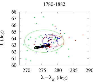
2.13Simulated and observed activity profile of visual size Quadrantids, ejecetd between 1780 - 1882 AD . . . 73
2.14Simulated and observed radiant position of visual Quadrantids, ejected between 1780-1882 . . . 74
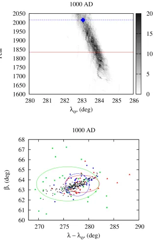
2.17Evolution of the descending nodes of visual size meteoroids, ejected from 2003 EH1between
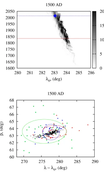
1000 AD and the present time . . . 78 2.18Evolution of the descending nodes of visual size meteoroids, ejected from 2003 EH1between
1500 AD and the present time . . . 79
3.1 Mean orbits of P/1999 J6, 96P/Machholz and mean daytime Arietids . . . 93 3.2 Backward evolution of the nominal orbital elements of comet P/1999 J6, along with 104clones,
over 2000 years. . . 96 3.3 Backward evolution of the nominal orbital elements of comet 96P, along with 104 clones, over
5×10⁴years. . . . 97
3.4 Past Kozai-type evolution of the orbit of 96P for 20000 years, across lines of different values of the Kozai energyC . . . 103 3.5 Assumed variability of meteoroid production rate for cases 5 and 7 in Table 3.2 . . . 105 3.6 Simulated activity profile of the daytime Arietids for meteoroid ejection from six different clones
for case 1. . . 107 3.7 Present distribution of the solar longitudeλof meteoroids, as a function of the ejection epoch
in the common era . . . 109 3.8 Weighted activity profile of the daytime Arietids as a function of the perihelion distance of the
parent during meteoroid ejection for case 1 . . . 110 3.9 Radiant position of the simulated daytime Arietids for case 1 in Table 3.2 and for clone (b) in
Fig. 3.8 . . . 111 3.10Distribution of the mean orbital elements of the Daytime Arietids as a function of the solar
longitude, ejected from clones of P/1999 J6 for case 1 . . . 112 3.11Simulated unweighted activity profile for the present daytime Arietids for meteoroid ejection in
case 6, for six different clones . . . 113 3.12Weighted activity profile for the daytime Arietids, at the present for meteoroid ejection from 96P
in case 6 in Table 3.2 for six different clones. . . 114 3.13Simulated distribution of the solar longitudeλof meteoroids, for six clones of 96P/Machholz,
as a function of the ejection epoch, for case 6 in Table 3.2 . . . 115 3.14Simulated and observed unweighted activity profile of the daytime Arietids for meteoroid
ejec-tion from 96P/Machholz for case 7 for six different clones . . . 117 3.15Present distribution of the solar longitudeλof meteoroids, as a function of the ejection epoch
for case 7 in Table 3.2 . . . 118
3.16Weighted activity profile of the daytime Arietids, at the present for meteoroid ejection from comet 96P/Machholz for case 7 . . . 119 3.17Simulated and observed radiant position of the daytime Arietids, for case 7 in Table 3.2 . . . . 120 3.18Distribution of the mean orbital elements of the Daytime Arietids as a function of the solar
longitude, ejected from clones of 96P/Machholz for case 7 . . . 121 3.19Simulated and observed unweighted activity profiles of the daytime Arietids for meteoroid
ejec-tion from comet 96P/Machholz for case 5 for six different clones . . . 123 3.20Present distribution of the solar longitudeλof meteoroids, as a function of the ejection epoch
for case 5 in Table 3.2 . . . 124 3.21Weighted activity profile of the daytime Arietids for meteoroid ejection from comet 96P/Machholz
for case 5 . . . 125 3.22Simulated and observed radiant position of the simulated daytime Arietids, for case 5 in Table 3.2 126 3.23Distribution of the mean orbital elements of the daytime Arietids as a function of the solar
longitude, ejected from clones of 96P/Machholz for case 5 . . . 127 3.24Distribution of the mean orbital elements of the simulated daytime Arietids as a function of the
solar longitude, ejected in 30000 BC (case 9) . . . 129 3.25Simulated and observed radiant position for meteoroids ejected in 30000 BC (case 9) from one
particular clone of comet 96P/Machholz . . . 130 3.26Distribution of the mean orbital elements of the simulated daytime Arietids as a function of the
solar longitude, ejected in 20000 BC (case 8) . . . 131 3.27Simulated and observed radiant position for meteoroids ejected in 20000 BC (case 8) from one
particular clone of comet 96P/Machholz . . . 132
4.1 Backwards time evolution of the ascending and descending nodes of the orbit of comet 96P/Machholz for one Kozai circulation cycle . . . 145 4.2 The orbits of comet 96P/Machholz and comet P/1999 J6. . . 148 4.3 Backward evolution of the nominal orbital elements of comet 96P/Machholz, along with 103
clones, over 5×10⁴years. . . . 153
4.4 Backward evolution of the nominal orbital elements of comet P/1999 J6, along with 103clones. . 155
4.5 Snapshot of the Kozai evolution of the orbit of 96P/Machholz for different values of the Kozai energyC . . . 156 4.6 Radiant distribution of meteoroids ejected from a single clone of comet 96P/Machholz, with
meteoroid ejection onset time 20000 BC . . . 161 4.7 Simulated, weighted and normalized activity profile of the Quadrantids, originating from 96P/Machholz162 4.8 Solar longitude distribution of Quadrantids as a function of meteoroid ejection from comet
96P/Machholz . . . 163
teoroid ejection from comet 96P . . . 165 4.11Simulated, weighted and normalized activity profile of the SDA, originating from 96P/Machholz 166 4.12Solar longitude distribution of SDA as a function of meteoroid ejection epoch, from comet
96P/Machholz . . . 167 4.13Simulated and observed radiant drift of SDA for meteoroid ejection from comet 96P . . . 167 4.14Simulated and observed distribution of the orbital elements of the SDAs for meteoroid ejection
from comet 96P . . . 168 4.15Simulated, weighted and normalized activity profile of the NDA, originating from 96P/Machholz 169 4.16Solar longitude distribution of NDA as a function of meteoroid ejection epoch, from comet
96P/Machholz . . . 169 4.17Simulated and observed radiant drifts of NDA for meteoroid ejection from comet 96P . . . 170 4.18Simulated distribution of the orbital elements of the NDAs for meteoroid ejection from comet 96P171 4.20Solar longitude distribution of filament 1 as a function of meteoroid ejection epoch, from comet
96P. . . 172 4.19Simulated, weighted and normalized activity profile of filament 1, originating from comet 96P . 173 4.21Simulated and observed radiant drifts of filament 1 for meteoroid ejection from comet 96P . . . 174 4.22Simulated and observed distributions of the orbital elements of filament 1 for meteoroid ejection
from comet 96P . . . 175 4.23Simulated, weighted and normalized activity profiles of filament 2, originating from 96P . . . . 176 4.24Solar longitude distribution of filament 2 as a function of meteoroid ejection epoch, from comet
96P. . . 177 4.25Simulated and observed radiant drifts of filament 2 for meteoroid ejection from comet 96P . . . 178 4.26Simulated and observed distributions of the orbital elements of the filament 2 for meteoroid
ejection from comet 96P . . . 179 4.27Simulated, weighted and normalized activity profile of filament 3, originating from 96P . . . . 180 4.28Solar longitude distribution of filament 3 as a function of meteoroid ejection epoch, from comet
96P. . . 180 4.29Simulated and observed radiant drifts of filament 3 for meteoroid ejection from comet 96P . . . 181 4.30Simulated distribution of the orbital elements of the filament 3 for meteoroid ejection from comet
96P. . . 182 4.31Simulated, weighted and normalized activity profile of filament 4 originating from 96P . . . 183 4.32Solar longitude distribution of filament 4 as a function of meteoroid ejection epoch, from comet
96P. . . 184 4.33Simulated and observed radiant drifts of filament 4 for meteoroid ejection from comet 96P . . . 185
4.34Simulated distribution of the orbital elements of the filament 4 for meteoroid ejection from comet 96P. . . 186 4.35Radiant distribution of meteoroids ejected from a single clone of comet P/1999 J6 . . . 187 4.36Simulated, weighted and normalized activity profile of the SDAs, originating from comet P/1999 J6188 4.37Combined simulated activity profile of the SDA, assuming meteoroid contribution from both,
96P and P/1999 J6. . . 189 4.38Solar longitude distribution of SDA as a function of meteoroid ejection epoch, from comet
P/1999 J6 . . . 189 4.39Simulated and observed radiant drifts of SDAs for meteoroid ejection from comet P/1999 J6 . . 190
4.40Simulated and observed distribution of the orbital elements of SDAs for assumed meteoroid ejection from comet P/1999 J6 . . . 191 4.41Simulated, weighted and normalized activity profile of filament 4 originating from comet P/1999 J6193 4.42Combined simulated activity profile of the filament 4 for meteoroid contribution from comets
96P and P/1999 J6. . . 194 4.43Solar longitude distribution of filament 4 as a function of meteoroid ejection epoch, from comet
P/1999 J6 . . . 194 4.44Simulated and observed radiant drifts of filament 4 for meteoroid ejection from comet P/1999 J6 195 4.45Simulated and observed distributions of the orbital elements of the filament 4 for meteoroid
ejection from comet P/1999 J6 . . . 196
A.1 Simulated, weighted and normalized activity profiles of QUA originating from comet 96P, for different initial meteoroid ejection onset times . . . 207 A.2 Simulated, weighted and normalized activity profiles of SDAs originating from comet 96P, for
different initial meteoroid ejection onset times . . . 208 A.3 Simulated, weighted and normalized activity profiles of NDAs originating from comet 96P, for
different initial meteoroid ejection onset times . . . 209 A.4 Simulated, weighted and normalized activity profiles of filament 1 originating from comet 96P,
for different initial meteoroid ejection onset times . . . 210 A.5 Simulated, weighted and normalized activity profiles of filament 2 originating from comet 96P,
for different initial meteoroid ejection onset times . . . 211 A.6 Simulated, weighted and normalized activity profiles of filament3 originating from comet 96P,
for different initial meteoroid ejection onset times . . . 212 A.7 Simulated, weighted and normalized activity profiles of filament 4 originating from comet 96P,
for different initial meteoroid ejection onset times . . . 213 A.8 Simulated, weighted and normalized activity profiles of SDAs originating from comet P/1999 J6,
for different initial meteoroid ejection onset times . . . 214
A.10Simulated, weighted and normalized activity profiles of SDAs, originating from P/1999 J6 and
96P, for different initial meteoroid ejection onset times. . . 216
A.11Simulated, weighted and normalized activity profiles of filament 4, originating from P/1999 J6 and 96P, for different initial meteoroid ejection onset times. . . 217
B.1 Illustration of the equatorial and ecliptic celestial reference frames . . . 220
B.2 Illustration of sun-centered ecliptic reference frame . . . 221
C.1 Illustration the orbital elements. . . 223
List of Tables
2.1 The osculating orbital elements of asteroid 2003 EH1, comet 96P/Machholz, comet 1490 Y1 and
the mean Quadrantid orbit . . . 45
2.2 Different variations of the "BJ98" (Brown and Jones, 1998) model . . . 50
2.3 Data for 8 high precision photographic Quadrantids, detected by the EMN . . . 52
2.4 Data for 5 high precision radar Quadrantids, observed by CMOR . . . 54
2.5 Average radiant position and dispersion of Quadrantid meteor shower, as detected by photo-graphic, video and radar techniques . . . 70
3.1 Various meteoroid ejection scenarios from P/1999 J6 . . . 100
3.2 Various cases used for meteoroid ejection throughout the forward simulations of comet 96P . . . 104
4.1 Geocentric characteristics of the meteor showers, possibly associated with the Machholz com-plex at their time of maximum activity. The columns denote: 1. The solar longitude of the start time of the activity profile, 2. The time of maximum activity, 3. The end time of the activity, 4. Sun-centered ecliptic longitude of the radiant, 5. Ecliptic latitude of the radiant, 6. Geocentric speed, 7. Geocentric equatorial right-ascension of radiant position in J2000.0. 8. Geocentric equatorial declination of the radiant in J2000.0. The remaining columns list the orbital elements at maximum activity. The superscript (a) indicates data obtained by CMOR, (b) corresponds to CAMS data, (c) observations derived by SAAMER and (d) corresponds to visual observations by IMO. . . 147
Appendix A Supplementary material to Chapter 4. . . 207
Appendix B Celestial reference frames . . . 218
Appendix C Orbital elements . . . 222
Appendix D Definitions . . . 225
List of Abbreviations and Symbols
AD From Latin “Anno Domini”. Refers to after Christ AU Astronomical Unit, equals to mean Sun-Earth distance BC Before Christ
CAI Calcium-Aluminum rich Inclusions CAMS Cameras for All-sky Meteor Surveillance CMOR Canadian Meteor Orbit Radar
Dec. Declination
DMS Dutch Meteor Society EN European fireball Network ESA European Space Agency FWHM Full-Width-Half-Maximum HTC Halley-Type comet
IAU International Astronomical Union IDP Interplanetary Dust Particle IMO International Meteor Organization
in-situ Latin word for “locally” or “on-site”
JFC Jupiter-Family Comet JPL Jet Propulsion Laboratory KBO Kuiper Belt Object
LONEOS Lowell Observatory for Near Earth Object Search LPC Long Period Comet
MAB Main Asteroid Belt MDC Meteor Data Center MMR Mean Motion Resonance
MOID Minimum Orbit Intersection Distance
NASA National Aeronautics and Space Administration NEA Near-Earth Asteroid
NEO Near-Earth Object R.A. Right Ascension
SAAMER Southern Argentina Agile Meteor Radar SOHO Solar and Heliospheric Observatory SOMN Southern Ontario Meteor Network SPC Short Period Comets
UT Universal Time ZHR Zenith-Hourly Rate
a Semi-major axis
α Celestial right ascension
αg Geocentric right ascension
A Cross-sectionorgeometric albedo
b Ecliptic latitude
β Ratio of solar radiation pressure to solar gravity
c Speed of light
CK orC Kozai energy
δ Celestial declination
δg Geocentric declination d Diameter
D0 Drummond’s orbital similarity criterion
DS H Southworth and Hawkins orbital similarity criterion e Eccentricity
Obliquity of the Earth’s equator to the ecliptic
φ Geographic latitude
Fe f f Effective force
FG Solar gravitational force FR Solar radiation pressure h Altitude
H Absolute visual magnitude
i Inclination km Kilometer
ξj Column vector of random numbers L Luminosity of the Sun
LZ The “Z-th” component of the orbital angular momentum
Λk j matrix of eigen-values
λ Geographic longitude
λ Solar longitude
λstart Solar longitude of the beginning of the activity profile
λmax Solar longitude of the maximum of the activity profile
λend Solar longitude of the end of the activity profile
λ−λ Sun-centered ecliptic longitude
mormo Mass of meteoroid M⊕ Mass of the planet Earth
M Mass of the Sun
mm Millimeter
µm Micrometer
ν6 Secular orbital resonance due to Jupiter and Saturn ω Argument of perihelion
Ω Longitude of the ascending node
P Orbital period
P(V−Ve j) Parabolic probability distribution of meteoroid ejection speeds q Perihelion distance
Q Aphelion distance
QPR Light scattering efficiency
rorro Heliocentric distance (Distance from the Sun) Rc Radius of comet nucleus
ρ Bulk density
ρc Bulk density of comet nucleus
σ Standard deviation
s Meteoroid radiusormass index
θ True anomaly
θc True anomaly of comet T Period of some periodic event
TJ Tisserand parameter with respect to Jupiter
Ve j Ejection speed of meteoroids from the surface of a comet Vobs Observed (in-atmosphere) speed of meteoroid
~
Vg Geocentric velocity vector
~
Vm Heliocentric velocity of meteoroid
~
VE Heliocentric velocity of the Earth V∞ Speed at “infinity”
worWs Weighting factor of meteoroids by their perihelion distance at time of ejection Wr Weighting factor of meteoroids by their size
X the “X” component of the heliocentric radius vector
˙
Y the “Y” component of the heliocentric velocity vector
Z the “Z” component of the heliocentric radius vector ˙
Z the “Z” component of the heliocentric velocity vector
Chapter 1
Introduction
The aim of this work is to explain the formation and past evolution of the interplanetary com-plex of bodies associated with comet 96P/Machholz. The goal is to obtain a self-consistent scenario of the fragmentation history of a single large progenitor, whose fragments and me-teoroid streams constitute the complex. We will concern ourselves with obtaining a broad coherent picture as to the relative contribution of these fragments to the associated meteoroid streams, and thus establishing the dominant parent body of the complex. In particular, we at-tempt to answer the question as to the earliest epoch when the first large progenitor might have been captured in a short period orbit, as a proxy of the age of the entire complex. For that purpose, we perform detailed modelling of the meteoroid streams, released from multiple par-ent bodies and fit our simulations to the observed showers characteristics, obtained by various meteor detection surveys (radar, photographic, TV and visual).
In the following sections we will review how meteoroids are related to their parents, and how they are liberated from comets and asteroids, and how a meteoroid stream is formed. Next, we will discuss what are the forces that meteoroids are subject to, upon release from a parent body, and how these particles evolve over time.
1.1
Small Solar System Bodies. Motivation
Asteroids, cometsandmeteoroids are leftovers from the formation of the Solar System about 4.6×10⁹years ago (e.g., Bouvier and Wadhwa, 2010), and are collectively known assmall Solar
System bodies(“small bodies” hereafter), to distinguish them from their larger counterparts, the planets. Over the history of the Solar System, the planets have been physically and chemically altered due to large-scale impacts, geological processes and weathering. Conversely, the small Solar System bodies are relatively pristine with little processing. Furthermore, the asteroids and comets have been extensively linked to the origin of life on the Earth. Shortly after the
planets had accreted most of their mass (∼4 billion years ago), their surfaces were constantly reshaped by heavy bombardments with the leftover debris of planet formation. It is believed that during that period water and carbon-based molecules may have been delivered on the Earth (Martins et al., 2013).
Without delving into a great detailed review of Solar System formation, a few key points should be noted in an attempt to outline the significance of the study of asteroids, comets and meteoroids. Asteroids are rock or metal based small bodies, believed to have condensed from the Solar nebula in the region of the terrestrial planets, Mercury, Venus, Earth and Mars (e.g., Bottke et al., 2006a; Crida, 2009). Observations suggest that some of the asteroids have been melted and differentiated (where heavier elements such as iron and nickel sunk to the center of the planetesimal, while lighter elements surrounded the core and formed the crust or the mantle of the asteroid). However, the bulk of the asteroids have never been heated to their melting point and are believed to be pristine and constitute a class of asteroids known as chondrites. These asteroids are made of three main components: Calcium-Aluminum rich Inclusions (CAI) (millimeter sized grains of refractory material - mostly Calcium and Aluminum), chondrules
(millimeter sized silicate spherules, 2 million years older than the CAI (e.g., Amelin et al., 2002; Bizzarro et al., 2004), and a matrix holding everything together. The chondrites are believed to be the key to understanding the early chemical composition and physical process of the early matter in the region of the terrestrial planets.
In contrast, comets are icy bodies with embedded solid dust particles within (Whipple, 1950, 1951). They are believed to have coalesced near the orbits of theGiant planets, Jupiter, Saturn, Uranus and Neptune (e.g., Fernández, 1997), where the temperatures were low enough to allow for volatiles to condense. The most important feature of the physical and dynamical evolution of the comets is that, unlike asteroids, the comets have never been heated up above 50 K, and thus are believed to have preserved even better the footprint of the primordial mixture in the region of the giant planets.
Dynamical models of the formation of the Solar System strive to understand the redistri-bution and evolution of the matter throughout the history of the Solar System, with the aim of establishing its locus of origin. Combined with ground-based observations or in-situ explo-rations this study provides crucial information as to the physical and chemical processes that took place 4.6 billion years ago.
1.1. SmallSolarSystemBodies. Motivation 3
1. The Chicxulub crater in the Yucatan peninsula. With dimensions more than 180 km wide and 20 km deep, the crater is believed to have formed in a catastrophic collision of the Earth with an asteroid about 66 million years ago (Renne et al., 2013). The event is associated with theCretaceous-Paleogenemass extinction event (the extinction of the dinosaurs) (e.g., Schulte et al., 2010).
2. The largest documented impact in the history of mankind is theTunguska event, in which a massive explosion on June 30, 1908 devastated ∼ 2000 km2 a remote forest area in Russia
(Ben-Menahem, 1975). The scientific investigations provide evidence for an explosion of a small asteroid or comet (a few tens of meters across) at an altitude of ≈10 km in the Earth’s atmosphere (Vasilyev, 1998). Kresak (1978) argued that the impactor may be a fragment of comet 2P/Encke, which is associated with the Taurid meteoroid complex (see Asher (1991) for an extensive review).
3. On February 15, 2013, a 20 meter size asteroid (Brown et al., 2013) entered the Earth’s atmosphere and exploded at an altitude of≈30 km over the Russian city of Chelyabinsk. Over 1000 people were reportedly injured by shattered windows due to the blast wave (Popova et al., 2013). The energy deposition in the explosion was estimated to be≈500 kilotons (Brown et al., 2013), equivalent to 20-30 times the energy released in the detonation of the Hiroshima atomic bomb. Silber et al. (2009) argued that the impact probability from objects in the size range 10 - 50 m, equivalent to the Chelyabinsk event asteroid is by an order of magnitude higher than initially thought.
Presently, scientists strive to constrain the size distribution, composition and orbits of the
Near-Earth Objects(NEOs) and understand their dynamics for numerous of reasons. For ex-ample:
1. Modelling of the dynamical evolution of small bodies may provide a crucial information as to the formation of the planets, their physical and dynamical evolution and the birth regions of asteroids and comets.
2. Determine a suitable candidate and time forin-situexploration via space mission. 3. Predict if a an object is moving on a collision course with the Earth, and develop mitiga-tion strategies.
Astronom-ical Union (IAU) assembly in 1958, adopted the definition of a meteoroid as: “A solid object moving in the interplanetary space, of a size considerably smaller than asteroid and
consider-ably larger than an atom” (Millman, 1961). That definition is vague and immediately raises the question “what is the lower limit of the term asteroid?”. Beech and Steel (1995) suggested that meteoroid should be defined as any solid interplanetary object with size greater than 100µm and less than 10 m. According to that definition, objects larger than 10 m are considered as-teroids, while particles less than 100 µm are regarded as dust particles. More recently, Rubin and Grossman (2010) proposed a new definition, where meteoroids should be considered in-terplanetary bodies with size between 10 µm and 1 m, where solid particles between 10 µm and 2 mm are referred to as micro-meteoroids. Any particle less than 10 microns is consid-eredInterplanetary Dust Particle(IDP). Although there is no a rigorous boundary between the size of a meteoroid and asteroid, the above definitions nevertheless provides a basic sense as to the size of these objects. Figure 1.1 illustrates the size and masses of some known objects, including the asteroids, comets and meteoroids.
1.2. Parent bodies of meteoroids 5
Meteoroid study is scientifically important for numerous of reasons, though the most im-portant ones within the scope of this work are:
1. Meteoroids are proxies of their parent bodies - the comets and asteroids (Sec. 1.2). For-tunately, comets and asteroids rarely intersect the Earth’s orbit, whereas our planet is constantly hit with small debris. The linkage of meteoroids to their parent is thus of a crucial importance. It allows us to sample their parent asteroids or comets from the Earth, whilein-situexplorations are generally expensive.
2. Even the smallest meteoroids approaching the Earth may pose a hazard to the Earth’s artificial satellites, where a hypervelocity impact could damage spacecraft components. In fact, on the night of August 12, 1993, astronauts on-board of theMirstation reported audible impact noise on the craft’s exterior, which was later verified that the space station had been hit by∼ 2000 meteoroids, which damaged the solar panels (e.g., Beech et al., 1995).
1.2
Parent bodies of meteoroids
1.2.1
Comets
We have briefly discussed in Sec. 1.1 that comets are icy bodies with embedded solid dust particles within and have formed in the region of the giant planets. However for a full under-standing of how meteoroids are related to comets, a few additional definitions and facts need to be presented.
An active comet consists of four distinct features - thenucleus, coma,dust tailandion or gas tail, respectively. Whipple (1950) suggested a comet model often referred to as thedirty snowballmodel or theicy conglomeratemodel, which describes a comet nucleus as irregularly shaped solid body consisting of a mixture of frozen volatiles with embedded dust particles within. Figure 1.2 shows an illustration of what a comet nucleus interior is believed to look like. Greenberg (1998) argued that roughly 26% of the nucleus mass is contained in refractory silicate particles, 23% in complex organic refractory material (dominated by carbon), and the remainder being occupied by frozen volatiles. The most abundant among the volatiles is the
∼ 30% with a mixture of other frozen gases such as, CO, CO2, CH3OH, CH4, NH, etc, each
contributing by about 2% by mass. At their reservoirs (Sec. 1.1), comets orbit the Sun in regions of extremely low temperatures, so the cometary ices are in solid state.
sub-Figure 1.2: Illustration of an assumed structure of a comet nucleus. Image credit:
http://explanet.info/Chapter14.htm
limation (direct transition of a solid ice into a gas) of the the frozen volatiles. The distance at which the cometary ices begin to sublimate is a strong function of the composition of the volatiles. Delsemme (1982) calculated that water ice can sublimate at a heliocentric distance (distance from the Sun) of ≈ 3 AU, whereas more volatile substances such as CO2 and CO
begin to evaporate even further, at distances beyond 5 AU. During sublimation, the escap-ing gas expands almost radially outwards, draggescap-ing away trapped dust particles of different size (submicron - centimeter sized), within the ice. Generally, the smaller particles are more abundant than millimeter and centimeter particles. Upon release, the particles are subjected to the minuscule nucleus gravity and Solar radiation pressure (Sec. 1.4.2) that is strictly size and mass dependent. The photon pressure drags the smaller (micron and sub-micron) particles radially opposite to the Sun’s direction, forming an extended envelope of gas and dust (micron sized particles), called thedust tailof the comet (see Fig. 1.3). The gas and dust surrounding the nucleus is referred to as thecoma. Furthermore, the Sun’s energetic UV radiation ionizes some of the coma atoms while the solar wind pushes the ions in direction opposite to the Sun, resulting in a narrow and long structure known as theion or gas tail. The released larger par-ticles (hundreds of microns to centimeter) are meteoroids and will be reviewed in Sec. 1.3 and Sec. 1.4.
1.2. Parent bodies of meteoroids 7
Figure 1.3: Illustration of the main components of an active comet. Image credit:https://lcogt.net
1P/Halley in 1986. That was the first ever direct imaging and measurement of comet’s nucleus size. The results showed that the size of the nucleus is roughly 15 km long, 7 km to 10 km wide and it was darker than previously thought, being covered by a thick layer of dust. Only about 15% of the nucleus surface was active. The estimated nucleus density was∼0.6 g.cm−3 (Sagdeev et al., 1988), with the mass of the ejected material being 80% water ice and 10% of CO. Figure 1.4 shows the sizes and shapes of a few comets which have been visited by spacecraft.
On November 12, 2014, for first time a space probe landed on comet surface. The Phi-lae lander, of the ESA’s Rosetta mission, made a successful touch on the surface of comet 67P/Churyumov-Gerasimenko.The preliminary results indicated that the surface of the comets is rich in carbon-based compounds and similar to other comets its surface is extremely dark with geometric albedo (the ratio of reflected to incident light) of A ≈ 0.06 (Capaccioni et al., 2015). Just for a comparison the latter value almost corresponds to a pure charcoal. Among other cometary missions are e.g., theDeep Impactmission to comet 9P/Temple, theStardust
mission with an aim of collecting dust from the coma of comet 81P/Wild.
Comet reservoirs and orbital classifications
Figure 1.4: Illustration of the shapes and sizes of some comets, visited by spacecrafts. Image credit:
1.2. Parent bodies of meteoroids 9
icy planetesimals in that region, were scattered away during that dynamical instability leaving only about 1% of the initial icy population beyond the orbit of Neptune (Morbidelli et al., 2005; Levison et al., 2008). Sometimes these objects are referred to astrans-Neptunian objects
(TNOs). Presently, this region is recognized as theKuiper belt(Edgeworth, 1949) or sometimes also called theEdgeworth-Kuiper beltwhich roughly extends from 35 AU - 50 AU (Stern and Colwell, 1997) (see also Fig. 1.5). It was named after the Dutch-American astronomer Gerard Kuiper, though he did not actually predict its existence. The Kuiper belt is believed to supply the short period comets (SPC), comets with orbital period of P < 200 years, into the inner Solar System.
Figure 1.5:Location of the Kuiper belt, relative to planetary orbits. Image credit:Pearson Education. Inc.
The rest of the scattered planetesimals during that instability period, were ejected out of the planetary region to nearly interstellar distances, where these comets form a spherical shell of 1012−1013comets, surrounding the Solar System. This shell is named theOort cloudafter the
Dutch astronomer, Ian Oort (Oort, 1950), who first hypothesized its existence.
pertur-Figure 1.6:Location of the Oort cloud, relative to planetary orbits. Image credit:Pearson Education. Inc.
bation by close passing stars, giant molecular clouds or galactic tides. These perturbations are thought as the mechanism of delivering the long-period comets (LPC), comets with periods (P > 200 years) into the planetary region (e.g., Duncan, 2008). The process is complicated and involves dynamical capture of these comets by the giant planets which are subsequently “handed-in” to the next planet, until its perihelion distance reaches a value below 5 AU (ap-proximately the extent of Jupiter’s orbit) where it can become an active comet.
1.2.2
Main Asteroid Belt
Most of the known asteroids (also referred to as minor planets) orbit the Sun between the orbits of planets Mars and Jupiter (see Fig. 1.7), or roughly between 2 AU and 4 AU, known as the Main Asteroid Belt (MAB hereafter). Their size vary greatly from a few kilometers to a few hundreds of kilometers. The largest asteroid is 1 Ceres(now referred to as a dwarf planet) which has a diameterd ≈950 km, followed by asteroids4 Vesta-d ≈525 km (Russell et al., 2012), 2 Pallas (Pitjeva, 2005) and 10 Hygiea. Presently estimated mass of MAB is
MMAB ≈ 5×10⁻⁴M⊕ (1 M⊕ ≈ 6×1024 kg is the mass of the Earth), where half of this mass
1.2. Parent bodies of meteoroids 11
mass of the belt is only 0.1% of the original mass (e.g., Petit et al., 2001), the bulk being ejected or accumulated by the planets.
The orbits of most asteroids in the MAB are relatively stable with a few regions which are heavily disturbed by the gravitational influence of Jupiter. In those regions the asteroids’ orbital periods are synchronously locked to the orbital period of Jupiter, a mechanism known
as a Mean Motion resonance (MMR hereafter). That is evidenced by apparent depletion of
asteroids in those regions, known as the Kirkwood gaps, which have been scattered away by Jupiter. These gaps are approximately found near heliocentric distances of 2.5 AU, 2.83 AU and 3.27, respectively, corresponding to 3:1, 5:2 and 2:1 MMR with Jupiter. An additional and more complex perturbing mechanism also responsible for asteroid scatter is theν6secular
resonance region, due to the combined perturbation by Jupiter and Saturn.
2 AU
Figure 1.7: Location of the Main Asteroid Belt, relative to planetary orbits. Image credit:
Delivery of asteroids to the near-Earth space.
Asteroids in these MMR regions are heavily perturbed by the Jupiter and Saturn and their orbital eccentricities are increased, so they attain orbits which may bring them to Venus and Earth-crossing orbits (Morbidelli et al., 2002). Once on such orbits, these asteroids are called
Near-Earth Objects(NEOs hereafter). Strictly speaking, NEOs are defined as having orbital perihelion distanceq< 1.3 AU and aphelion distanceQ> 0.983 AU.
Once in the planetary region, the dynamical evolution of NEOs is controlled by Jupiter and to a lesser degree by close encounters with the terrestrial planets. The dynamical lifetime of NEOs is shorter than the age of the Solar System, so the fact that we still observe them today strongly suggests that they are replenished (Gladman et al., 2000; Morbidelli et al., 2002). Numerical simulations indicate that the majority of the NEOs are supplied from the MAB, while only≈6% originate from Jupiter Family Comets (JFCs) (Bottke et al., 2002). However, as discussed in Sec. 1.2.2 the resonance regions in the MAB are almost depleted, so there must be a way of transporting asteroids from nearly stable orbits to these “escape hatches”.
It has been shown that radiation forces from the Sun, such as the Yarkovsky effect (see e.g., Bottke et al., 2006b) can increase the orbital semi-major axis, and once the body reaches these resonance regions, it may well be injected in the terrestrial planets region. It’s been demonstrated that the Yarkovsky effect is an efficient mechanism of pushing meteoroids and asteroids (up to 10 km in size) to these “escape hatches” and subsequently producing NEOs (Bottke et al., 2000; Vokrouhlický and Farinella, 2000; Morbidelli et al., 2002). It is noteworthy that the Yarkovsky effect was measured for first time in 2003 for the near-Earth and potentially hazardous asteroid 6489 “Golevka” (Chesley et al., 2003).
1.3
Formation of meteoroid streams
1.3.1
Cometary origin
Presently, formation of cometary meteoroid streams is a relatively well understood process (e.g., Whipple, 1951; Kresak, 1976; Williams, 1992; Vaubaillon et al., 2005). The break-through in understanding this process originated from Whipple’s icy conglomerate model of comet nuclei (Whipple, 1950).
1.3. Formation of meteoroid streams 13
and Richter, 2005), whereas CO2roughly begins to sublimate atr ≈5 AU. However, generally
the abundance of these gases are low compared to the water ice (Greenberg, 1998), and most likely the evaporation of these ices lifts up only the smallest particles off the surface of the comet. In order for larger particles to be lifted and accelerated, more violent cometary activ-ity is expected. Generally, meteoroid production is associated with sublimation of water ice, roughly corresponding tor=3AU, partly due to the greater gas production rate and the greater molecular weight of the water vapor. In fact, a particle can only leave the surface of the comet if the gas drag force overcomes the nucleus gravity. A typical upper limit as to particles’ sizes, released by water sublimation from comets is a few tens of centimeters. The latter is a strong function of the particle’s size and density which may vary anywhere betweenρ = 500 kg.m−3 for ice particles toρ =3000 kg.m−3for silicate particles.
Ejection speeds
When the particles are ejected from the comet nucleus the gas drag accelerates the particles approximately radially outward from the nucleus. At about ten nucleus radii the particles reach a terminal speed, which typically does not exceed 1 km.s−1. A that point the particles follow a
trajectory independent of the parent and are referred to as meteoroids (see also Sec. 1.1).
The magnitude of the ejection speed is strictly a function of the heliocentric distance, the size of the nucleus as well as the size and density of the ejected particle. As a result of his icy-conglomerate comet model, Whipple (1951) derived for the ejection speed of a spherical particles, the expression:
Ve j ≈ 8.3r
−1.125
R1c/2m
−1/6ρ−1/3
f, (1.1)
whereVe j is the ejection speed of the meteoroid in m.s−1, r is the heliocentric distance in
AU, Rc is the radius of the comet nucleus in km, m is the mass of the meteoroid in grams,
ρ is the bulk density of the meteoroid in (g.cm−3) and f is the fraction of the solar radiation
available for sublimation (usually taken as unity). Using the above expression for a typical meteoroid, equivalent to a visual meteor, ofρ = 0.7 g.cm−3 and mass ofm= 3×10⁻³ grams, ejected from a comet nucleus of sizeRc = 5 km at a heliocentric distance of r = 1 AU, the
magnitude of the ejection speed isVe j ≈ 55 m.s−1.
Ve j ≈10.2r
−1.038
R1c/2m
−1/6ρ−1/3
f, (1.2)
where the variables are the same as in Eq. 1.1. The only difference in the latter equation is the modified dependence on the heliocentric distance, though the overall magnitude of the ejection speed does not differ much from Whipple’s expression. Indeed, using the same values for the meteoroid size and density and size of the comet as in Eq. 1.1 the resulting ejection speed isVe j ≈67 m.s−1.
Over the last decades there have been several revisions of the Whipple’s original expres-sion, with accounting for various effects. Gustafson (1989a) explored the ejection speeds as a function of the meteoroids’ shape, considering particles of “flakes” and “needle”-like shapes. Hughes (2000) considered the scenario that ejected meteoroids contain frozen ices where upon particle ejection, the residual ices may continue to sublimate and produce a “rocket”-like force increasing the speed of the meteoroid. However, the overall result would agree that the ejection speeds are small and are less than the speed of the escaping gas (less than 1 km.s−1) (Hughes, 2000).
The heliocentric (orbiting the Sun) speed of a body is given by:
Vh = s
GM
2
r −
1
a !
, (1.3)
whereGis the standard gravitational constant in units (m3kg−1s−2), M≈2×1030kg is the
mass of the Sun,ris the heliocentric distance of the body in meters andais the body’s orbital semi-major axis in meters (see Appendix A for definition of the orbital elements). Assuming a comet with orbital semi-major axis of a = 3 AU (a typical value for JFC), located at a heliocentric distance ofr = 1 AU, its heliocentric speed will beVh ≈47 km.s−1. We compare
that speed to the ejection speedVe j ≈50 m.s−1of a s =1 mm meteoroid of massm =3×10⁻³
grams, from the surface of a comet of radiusRc = 5 km at a heliocentric distance ofr =1 AU.
1.3. Formation of meteoroid streams 15
planets as well as non-gravitational forces (Sec. 1.4).
Evolution of comets into asteroids
Levison and Duncan (1997) calculated that the physical lifetime of short-period comets is
∼ 12000 years, which is significantly lower than their dynamical lifetime∼ 4.5×10⁷ years.
That implies that cometary nuclei “fade” (disappear due to a breakup or become inactive) before they are ejected from the inner Solar System. Whitman et al. (2006) argued that there is a greater probability of a comet nucleus becoming inactive rather than being completely disrupted. There a few mechanisms that are believed to lead to “demise” of comets.
1. Weissman et al. (1989) argued that comets lose roughly 0.01 - 0.1% of their mass on each perihelion return. Thus, cometary activity can not be sustained indefinitely, especially active comets. Eventually, over many revolutions around the Sun, the cometary volatiles will deplete and only refractory inert material will remain (e.g., Whipple, 1950; Weissman et al., 1989). Weissman (1980) estimated lifetimes of∼600, 4500, and 4×10⁵returns for 1 km radius water ice spheres with surface albedo of 0 and density of 0.6 g.cm−3, for long-period comets with perihelia of 1, 2, and 3 AU, respectively. The lifetimes of short-period comets will be lower due to their lower semi-major axis and eccentricity. Observationally, the “dead” comet nucleus will be dark indistinguishable from an asteroid. This is referred to as anextinct comet. However, the complete de-volatilization of a comet nucleus is not a well understood process. Weissman (1980) argued that comets are likely to develop an inert crust (see below) of their surface, which would prevent further sublimation and thus subsequent lost of volatiles.
2. Another mechanism which may lead to low or no cometary activity is development and inert crust (mantle) on the surface of a comet. This mechanism was proposed by Whipple (1950) as a consequence of his “icy-conglomerate nucleus” model. Rickman et al. (1990) noted that during cometary activity only the lightest particles can escape the nucleus gravity. The larger silicate particles and boulders remain on the surface or are lifted up and eventually fall back onto the surface. Over time, this material will form a “blanket” of inert crust on the cometary surface, suppressing or ceasing the activity. This is referred to as adormant comet. Similar to the case with extinct comet, the nucleus of a dormant comet would be difficult to be differentiated from an asteroid. However, occasionally a passage of dormant comet close to some of the planets, the tidal forces may produce cracks in the mantle which may reactivated the comet for a short time (Jenniskens, 2006).
% of the NEO population (Fernández et al., 2001; Bottke et al., 2002).
1.3.2
Asteroidal origin
Presently, there are only two meteor showers associated with asteroids. The core of the Quad-rantid meteoroid streams is asteroid 2003 EH1 (e.g., Jenniskens, 2004; Wiegert and Brown,
2005; Neslušan et al., 2013), whereas the Geminids meteor shower has been linked to asteroid 3200 Phaeton (Gustafson, 1989b; Williams and Wu, 1993; Ryabova, 2016). However, the ex-istence of dormant or extinct comets (Sec. 1.3.1) makes it difficult to link meteoroid streams to asteroids, for one obvious reason: A comet may have produced a meteoroid stream in the past, during its active period (see Sec. 1.3.1), and later has become dormant or extinct. If the stream is not tremendously old, the particles can still be linked to the parent body. But the parent will presently be dormant and thus it will be recognized as an asteroid which will lead to association of the resulting stream with an asteroid.
Although, there have been a number of studies (e.g., Steel, 1995; Jopek et al., 2002; Porubˇcan et al., 2004) dedicated to establishing a child-parent relationship of meteoroid stream with an asteroid, the subject is still debatable. Nevertheless, below is presented a few mecha-nisms which may lead to mass shedding from the surface of an asteroid.
Mass loss from asteroids
1. Collision- In 2010, a peculiar object was discovered, named P/2010 A2, showing evidence of mass loss. Computed orbital elements revealed that the object is a member of the MAB (Jewitt et al., 2010). Furthermore, observations of the near nucleus environment suggested that the mass loss is different from cometary water-ice sublimation. Follow-up calculations of dust and fragment dispersal indicated that the mass loss was likely due to a collision with another body, results consistent with the mean asteroid velocity dispersion in the MAB (∆V ≈5 km.s−1)
(Bottke et al., 1994) and with models of catastrophic collision between rocky bodies (Benz and Asphaug, 1999). However, the work of Benz and Asphaug (1999) suggests that the ejection speeds of fragments in a collision are low and thus a direct injection of meteoroids from the MAB into Earth-crossing orbit is unlikely.
1.4. Dynamical evolution of meteoroid streams 17
may explain the lack of fast rotating asteroids of size∼10 km, suggesting that they disintegrate when they reach the spin limit∼2.2 hours (Pravec et al., 2002). Thus, all fast rotating asteroids with absolute magnitude of H<22 (roughly 150 m) must be monolithic (Pravec et al., 2002). This mass-shedding mechanism is also believed to produce the observed binary asteroids (e.g., Walsh et al., 2008), which account for 15% among the NEO and MAB population. The YORP spin-up was measured for first time in 2007 for near-Earth asteroid 2000 PH5 (Lowry et al., 2007).
Finally, it is not clear whether the above mentioned mechanisms can explain the formation of the Geminids or the Quadrantids. We recall that, Gustafson (1989b) showed that the activity of Geminids can be explained if Phaeton was an active comet ∼ 1000 years ago and then it gradually ceased activity. Similar work was done by Abedin et al. (2015) who showed that the timing and duration of the core of the Quadrantids can be explained by cometary activity from the surface of 2003 EH1some 200 years ago, which later similar to Phaeton perhaps has gone
dormant or extinct.
1.4
Dynamical evolution of meteoroid streams
1.4.1
Gravitational and secular evolution
All Solar System bodies move under the dominant central force of the Sun, with planets acting as perturbers. Hence, the orbits of the bodies to a first approximation are Keplerian (the two body problem), with planets impinging small but significant disturbances on their Keplerian motion (the N-body problem). The most massive planet in the Solar System is Jupiter, so it is expected to be the main perturber, where Saturn, Uranus and Neptune will also have a substantial effect. In addition, smallest meteoroids (micrometer - centimeter) will be also affected by non-gravitational forces (see Sec. 1.4.2).
It is well known fact the the N-body problem is not integrable in analytic functions (in a closed form), though the motion of a body can be approximated as infinite series of polynomials (Murray and Dermott, 2000). Simulations of the dynamical evolution of meteoroid streams in the past were performed by hand, where the myriad of particles (meteoroids) were replaced by a few particles only (Williams, 1992). Often scientists had to resort to analytical secular methods, where the gravitational influence of the planets were averaged over a complete orbit. Nowadays with the advancement of computational technologies these tasks are easily achievable and the problems can be solved numerically.