Phased Array Calibration by Binary Compressed Sensing
Galina Baburs1, *, Diego Caratelli2, 3, and Arman Mirmanov4
Abstract—This paper presents a calibration technique for phased array radars. The real embedded patterns of the array elements are measured independently in operating mode, while taking antenna coupling and other parasitic effects into account. The proposed technique does not affect the operation of the antenna array. The use of suitable switches integrated in the beamforming network of the array allows introducing sparsity into the measured summed signal. This enables the extraction of the angular dependent calibration coefficients by means of a dedicated compressed sensing approach.
1. INTRODUCTION
Coupling phenomena occur, to some extent, in all antenna arrays, and can significantly affect their operation [1–6]. Accurate calibration is key to preserve and control the main beam direction and shape, as well as the sidelobe levels of a radar antenna [7–9]. In practice, the beamforming network of an antenna array is often affected by electronic drift, as well as temperature and environmental conditions; thus, calibration of a fielded radar system is required [10]. In this context, it is beneficial to have the capability of performing calibration while the system is in operating mode.
In this work we present a technique for the calibration of phase and amplitude errors introduced at antenna element level in phased array radars with beamforming on receive. The technique is implemented in the operating mode of the radar. In this way, the measured patterns include the effect of mutual antenna coupling and other parasitic effects. No separate measurements of the embedded radiation patterns or coupling level between array elements are required.
We consider a radar system consisting of an array of identical antennas under the assumption of a narrowband sounding signal. We assume that the rest of the hardware operates in ideal manner. The signal processing relies on pulse compression of the processed signals.
As known, the calibration of a phased array antenna while the device is in service can be a complex and time-consuming procedure which limits the use or imposes an unacceptable overhead on the system [11]. On the other hand, the proposed technique is directly implemented in operating mode and, therefore, does not have the aforementioned drawbacks thanks to the adoption of a suitable signal processing procedure in combination with controlled time delays in the receiver channels.
During the calibration process, the extracted antenna correction coefficients are evaluated for all the array channels and for each specified angular direction. The number of measurements is minimized by using a compressed sensing (CS) approach. Sparsity is introduced into the aggregated received signals according to assigned binary delay vectors which specify the position of switches integrated in the beamforming network of the array. The sparsity property allows reconstructing the real (non-ideal) embedded patterns of the individual array elements in a computationally effective way by means of a
l2-minimization. Once the real patterns in operating mode are evaluated, the received signals along the various radar channels can be corrected (calibrated).
Received 29 May 2018, Accepted 23 August 2018, Scheduled 6 September 2018 * Corresponding author: Galina Babur ([email protected]).
The paper is organized as follows. Section 2 describes the received signal model. The calibration technique is presented in Section 3. Considerations on the application of the proposed calibration technique are reported in Section 4. The numerical results which demonstrate the effectiveness of the presented calibration technique are discussed in Section 5. The concluding remarks can be found in Section 6. Section 7 contains the conclusions.
2. RECEIVED SIGNAL MODEL
A phased array is a structure consisting of multiple antennas whose effective (summed) radiation pattern can be controlled by phasing the signals of the individual elements. In the case of a linear phased array, the ideal received signal can be written as:
sR,0(t, θ) =
N
n=1
P0(θ)·e−j k(θ)·x(n)·s(t), (1)
wheres(t) is the complex envelope of a sounding signal suitable for pulse compression;N is the number of receiving elements; ¯kis the wavevector; ¯x(n) denotes the position vector of thenth receiving element for n ∈ [1, . . . , N]; θ is the angular position of a hypothetic target. In our work, we assume a linear frequency modulated (LFM) waveform for the sounding signal.
In real-life scenarios, the array elements display non-ideal embedded patterns Pn(θ) for n = 1,2, . . . , N. As a matter of fact, the signal received by each array element can be affected by multiple transmissions between antennas due to spurious mutual coupling processes [2, 6, 12]. Furthermore, the embedded radiation patterns can be distorted by non-idealities in the phase shifters embedded in the beamforming network, edge diffraction phenomena, as well as by impedance mismatches, and structural variations in elements themselves. Our calibration technique takes all of these effects into account since it is implemented in the operating mode of the radar under test.
The coupling between the elements of the considered N ×1 phased array can be modeled as a
symmetric N×N coupling matrix R [6, 7] with entriesR(n, m) =
1 n=m
rn,m n=m. The beamforming
of the array is performed along the angular direction θ0 which is assumed to identify the location of a known point target used for calibration, that is θ = θ0. Obviously, for a given angular direction the signal described in Eq. (1) becomes a function of time only. So, the actual signal received by the n-th antenna element can be written, in the absence of noise, as [6]:
snR,θ0(t) =
N
m=1
Pm(θ0)·rn,m·e−j k(θ0)·(x(m)−x(n))·s(t), (2)
where the index m is used for the modeling of coupling effects, while the indexn denotes the general receiving element. As can be noticed, because of the parasitic coupling processes, the signal received by then-th array element in Eq. (2) is influenced by the radiation patterns of all theN antennas forming the array. The exponents e−j k(θ0)·(x(m)−x(n)) (for m = 1, . . . , N) represent the propagation path term between the n-th antenna and all the array elements including the element itself (one of the values m
is equal to n). The self-coupling coefficient as well as the propagation path term of the n-th antenna element relative to itself (m=n) are both equal to one. So, Eq. (2) can also be recast as follows:
snR,θ0(t) =
⎛
⎝Pn(θ0) +
m=n
Pm(θ0)·rn,m·e−j k(θ0)·(x(m)−x(n))
⎞
⎠·s(t). (3)
The summation term in Eq. (3) measures the impact of the mutual coupling on the individual array element pattern Pn(θ0). It is apparent that the real radiation pattern of the n-th array element is described by the expression:
A(n, θ0) =
N
m=1
The finality of the proposed calibration process is to evaluate the coefficients described by Eq. (4) for
n= 1, . . . , N. By using these coefficients, Eq. (2) can be written as:
snR,θ0(t) =
A(n, θ0)
P0(θ0) ·P0
(θ0)·s(t). (5)
As known from the literature, the array pattern characteristics are affected by the errors on phase and amplitude of the radiated/received signals [13]. The ratio A(n, θ0)/P0(θ0) in (5) quantifies the relative error introduced on the ideal received signal, see Eq. (1). The original (ideal) patternP0(θ) is supposed to be known a priori. Once the coefficients A(n, θ0) are estimated, the received signal snR,θ0 can be readily corrected (calibrated).
We note here that our technique does not require a separate estimation of the coupling matrix.
3. CALIBRATION TECHNIQUE
The idea behind the proposed calibration technique is to equip the channels of a phased array radar with identical time delay lines controlled by suitable switches (see Fig. 1). The time delayδtis inversely proportional to the sounding signal bandwidth ΔF, that isδt= 1/ΔF, or its multiples. The controlled time delays are identical and do not depend on the number of radar channels contrary to the calibration technique in [14], which makes use of an element-wise off-setting in the receiving channels. In the case of large phased arrays with reduced operating bandwidth, the relative time offsets would result in too long time delays along the radar channels, that is impractical from an application standpoint. On the other hand, the here-proposed technique does not impose restrictions on the array size or the signal bandwidth, because the time delays introduced in the radar channels are the same. This allows overcoming the main limiting factor in the practical implementation of [14]. In this way, the developed calibration technique can be applied to small, medium, as well as large phased arrays.
For a waveform s(t) with large BT-product, the offset δt is small compared to the pulse duration. Though time or frequency offsets introduced into the signals can affect the array radiation pattern [15, 16], the chosen time delays do not influence the estimated angular-dependent coefficients
A(n, θ0) (real patterns) in Eq. (4) for the reasons detailed hereafter. Before pulse compression, the phase shift associated with the offset δt, at a given frequency f, can be written as Δϕ= 2·π·f·δt. After pulse compression, when the full bandwidth ΔF of the signal is to be accounted for, the actual phase shift becomes Δϕ = 2·π·ΔF ·δt, which is equal to 2·π or 0. Therefore, the time offset δt
Matched filter s(t)
0 , R
s
1 0 θ 2 3 0θ θ0 θ0
N
S
Point target used for calibration θ t δ0 1 0 1 1 0 1
t
δ δt δt
The angular direction of a point calibration target is equal to the beamformed angular direction, θ = θ .0
. . .
. . .
θ (t)
χθ0(τ) = χ
0 θ(τ ) +
1
1 χθ0(τ ) 2
2
is a binary delay vector
d = [d (1), ..., d (N)]
Figure 1. Phased array receiver with the introduced time delays.
1
y y2
0
θ θ0
i = round (τ/δt) 0 1 1 y 0 θ 2 y 0 θ
=
χθ0(τ = 0)χ
0
θ(τ = δt)
selectively applied to the received signal components does not result in any phase difference between the signals after their pulse compression. It is worth, also, stressing the point that the considered phase shift does not depend on the observation angleθ0.
We notice here the fact that the time shift δt= 1/ΔF is the minimal time interval which makes the signals separable after the relevant pulse compression. Since the signals can be separated, it is apparent that the introduced relative time shift ensures orthogonality between shifted and non-shifted signals in spite of the fact that they are highly overlapped in time. The orthogonality, as well as the phase alignment, between shifted and non-shifted signal components is the key property which makes the implementation of the proposed calibration technique possible.
The state of the switches along the receive channels is specified by a binary delay vector
d = [d(1), d(2), . . . , d(N)], d(n) ∈ (0,1) for n = 1,2, . . . , N, where 0 means no time delay, and 1 is associated with the time delay δt. To build the set of equations useful to the evaluation of the real pattern coefficients, different delay vectorsdare to be considered. Together they form a delay matrixD. Following the application of the selected time delays to the various received array signal contributions, the aggregated received signal can be written as follows:
sR,θ0(t) =
N
n=1
A(n, θ0)·s(t−d(n)·δt), (6)
where A(n, θ0) denotes the real embedded pattern of the general array element that accounts, also, for spurious antenna coupling phenomena and other parasitic effects. The knowledge of the actual embedded element patterns is instrumental in aligning the real array response to the ideal one, which is known a priori as per Eq. (1).
The matched filter output can be easily written in terms of the offset auto-correlation functions
ACFS of the signals(t), that is:
χθ0(τ) =
N
n=1
A(n, θ0)·ACFS(τ −d(n)·δt). (7)
The auto-correlation function allows the filtering process in time domain in analogy with the discrete delta function. In this case, the matched filter output can be written in the domain of the discrete time as:
χθ0(i) =
N
n=1
A(n, θ0)·d(n) +
N
n=1
A(n, θ0)·(u(n)−d(n)), (8)
wherei= 0,1,u is a unit vector (u(n) = 1,n= 1, ..., N) of the same dimension asd.
y1
θ0
yθ20
=
χθ0(i= 0)
χθ0(i= 1)
. (9)
The summation in Eq. (8) is equivalent to the integration of the products Aθ0(n) · d(n) and
Aθ0(n)·(u(n)−d(n)). The evaluation of the output signal allows the simultaneous measurement of the two quantities (see Fig. 2). The measured values are given by the two following inner products:
yθ10 yθ20
=
Aθ0,d
Aθ0,d
, (10)
where Aθ0 is a N-valued vector which contains the values of the real embedded patterns of the array elements along the angular direction θ0, whiled and d denote the delay vector (the set of binary test functions) and its complementary version, respectively.
To reconstruct the [N ×1] vector Aθ0 along each angular direction of interest θ0, we make use of a compressed sensing (CS) approach by performing L measurements, with L < N. This is possible thanks to the sparsity of the binary delay vectors d and d. The maximal sparsity of these vectors is evaluated asK =truncate(N/2). This condition is achieved when the numbers of ones and zeros ind
The coefficientsA(n, θ0) (which describe the real embedded patterns affected by the antenna mutual coupling effects) are estimated by means of a l2-minimization.
We stress here that the real pattern coefficientsA(n, θ0) are estimated in the operating mode of the considered phased array radar. This means that the calibration technique can properly model all the non-idealities, such as wave diffraction processes, impedance mismatch of the antennas, manufacturing tolerances, that affect the embedded element patterns Pn(θ0). Therefore, the estimated real patterns
ˆ
A(n, θ0) intrinsically include the effect of said undesired phenomena.
Based on Eq. (5), the correction (calibration) coefficient for the beamformed angular direction θ0 and n-th receive channel can be written as
C(n, θ0) = P0 (θ0) ˆ
A(n, θ0)
. (11)
The calibration process of the aggregated received signal in the operational radar mode is described by the following equation:
scorrR,θ0(t) =
N
n=1
C(n, θ0)·snR(t), (12)
where the superscript ‘corr’ stands for corrected.
4. APPLICATION OF THE PROPOSED CALIBRATION TECHNIQUE TO PHASED ARRAYS WITH ARBITRARY TOPOLOGY
Though the theory presented in Sections 2–3 describe the signal model and calibration technique for a linear phased array, here we show that the calibration principle can be extended to other types of arrays based on different beamforming algorithms. In the general case, the signal received by one array channel can be written, in analogy with Eq. (2), as:
snR,θ0,ϕ0(t) =
N
m=1
Pm(θ0, ϕ0)·rn,m·e−j k(θ0,ϕ0)·r(m)·wn·s(t), (13)
where (θ0, ϕ0) is the angular position of a point target used for calibration;r(m) = (xm, ym, zm) denotes the position vector of themth receiving element,m= 1, . . . , N;w(n) denotes the complex beamforming coefficient relevant to thenth receiving channel.
In this way, the real radiation pattern of thenth array element along the angular direction (θ0, ϕ0) can be described by the following time-invariant expression:
A(n, θ0, ϕ0) =
N
m=1
Pm(θ0, ϕ0)·rn,m·e−j k(θ0,ϕ0)·r(m)·wn. (14)
The introduced time delay d(n) does not influence the estimated angular-dependent coefficients
A(n, θ0, ϕ0) because the phases of the signals s(t) and s(t−d(n)) (shifted and non-shifted signals in the samenth channel) remain unchanged, as highlighted in Section 3.
Enforcing the proposed delay vectors does not result in an alteration of the array output, since the introduced delays do not change the signal phase (2π-phase shift is equivalent to no phase shift). On the other hand, after pulse compression, the signal in Eq. (13) received by the nth channel contributes to the aggregated signal at the discrete time instant i= 0 or i= 1 depending on whether d(n) = 0 or
d(n) = 1, respectively (see Fig. 2).
5. MODELING RESULTS
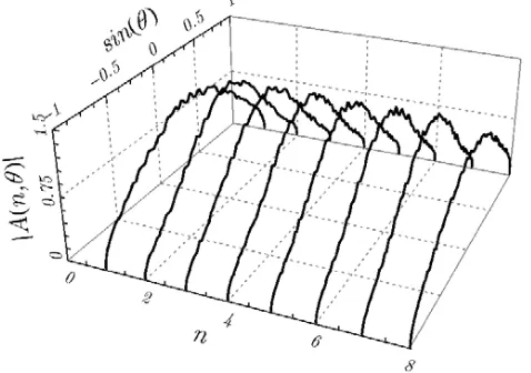
The modeling results relevant to the coefficients Aθ0 used for phased array calibration in receive mode are presented in this section for two uniform linear and circular array topologies. The carrier frequency is equal tof0= 10 GHz. We assume the coupling level to beρbetween adjacent antennas, and 0 between farther elements of the array. The radiation patterns of the antenna elements are described by cos(θ) and (1+ cosθ)/2 for the linear and circular array, respectively. The duration of the sounding LFM-signal and the relevant bandwidth are equal to 250µs and 40 MHz, respectively. We applied additive Gaussian noise to the signal s(t) in each receiver channel. No window weighting has been applied.
The first example (Figs. 3–6) is presented for a linear uniformly spaced array of N = 8 antennas separated by half-wavelength at the carrier frequency. Fig. 3 shows the embedded antenna radiation patterns when being affected by a parasitic coupling level ρ = 0.2, as well as by random amplitude and phase distortions of the excitation coefficients. The additive Gaussian noise has 5% variance in each receiver channel. We note here that the pulse compression by matched filter results in a noise suppression by a factor equal to the signal BT product, which is 10000 in our example. Furthermore, during the calibration process, the N antenna signals are divided into two groups (defined by the assigned delay vector) to be summed coherently in two different range cells (τ = 0 and τ =δt). This provides additional noise suppression by a factor N/2.
The measurement delay matrix [L×N] consists of L= 4 binary delay vectors d which specify the position of the switches in the array frontend for each measurement. For the experiment we used the following delay matrix:
D=
⎡ ⎢ ⎣
1 1 1 1 0 0 0 0 0 1 1 1 1 0 0 0 0 0 1 1 1 1 0 0 0 0 0 1 1 1 1 0
⎤ ⎥ ⎦.
For each angular directionθ0, four binary delay vectors (identified by the rows of the matrix) are applied consequently. Thus, the four signal levels measured consequently at the matched filter output at the time instantτ = 0 correspond to the delay matrixD, whereas the four signal levels measured at the time instant τ = δt correspond to the complementary delay matrixD. The concatenation of the matrices
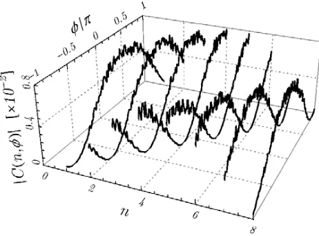
D and D results in the complete [N ×N] delay matrix. Fig. 4 shows the calibration coefficients
C(n, θ0) for the linear array obtained by making use of Eq. (11), for each angular direction and for each array element. Using the calculated calibration coefficients, we can recover the real embedded patterns (see Fig. 5) of the array elements forn= 1, . . . , N, by applyingl2-minimization. In turn, the
Figure 3. Array elements patterns influenced by the couplingρ= 0.2, as well as, by the amplitude and phase errors.
Figure 5. Corrected patterns of the linear array elements C(n, θ0)·A(n, θ0).
Figure 6. Ideal, non-calibrated and calibrated patterns of the circular phased array.
Figure 7. Array elements patterns influenced by the couplingρ= 0.3, as well as, by the amplitude and phase errors.
Figure 8. Calibration coefficients C(n, θ).
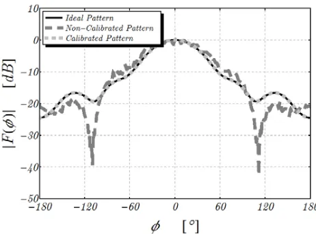
corrected embedded patterns contribute to the corrected array pattern, which is shown in Fig. 6 and here compared against the ideal and non-calibrated patterns for θ0 = 0 beamforming direction.
The second example (Figs. 7–10) is related to a circular phased array consisting ofN = 8 antennas. The diameter of the array is selected in such a way that adjacent elements are separated by half-wavelength at the working frequency. The embedded antenna radiation patterns are affected by a parasitic coupling levelρ= 0.3, as well as by random amplitude and phase distortions of the excitation coefficients (Fig. 7). The additive Gaussian noise has 10% variance in each receiver channel. The same delay matrixD consisting of the binary delay vectors has been applied to control the switches as in the first example. For each angular direction θ0, four binary delay vectors are applied consequently. The array calibration coefficients are estimated using Eq. (11) and are shown in Fig. 8 for the individual array channel. The obtained calibration coefficients are applied to the embedded patterns for their correction (Fig. 9). In turn, the corrected embedded patterns aggregate into the array pattern, which is shown in Fig. 10 and here compared against the corresponding ideal and non-calibrated patterns.
Figure 9. Corrected patterns of the circular array elements C(n, θ0)·A(n, θ0).
Figure 10. Ideal, non-calibrated and calibrated patterns of the circular phased array.
6. REMARKS
• The application of the proposed calibration technique is not limited by the size of the considered phased array. It can be applied to small, medium, as well as large phased arrays.
• The calibration principle can be applied to phased arrays having different topologies. It can be applied to 1D, 2D, as well as 3D (conformal) array structures [17–19].
• The proposed calibration technique can be applied to radar systems employing pulse compression, under the assumption that the time-bandwidth product of the sounding signal is much larger than 1. • Optimal results are achieved when sounding LFM signals having large BT product are used. Large values of the BT product reduce the impact of the noise on the measurements. The influence of the LFM signal range sidelobes on the measured values is negligible.
• The calibration technique is suitable for active, as well as, passive phased array radars.
We note here that the proposed calibration technique does not rely on the application of window weighting to the processed signals. However, this does not prevent the use of window functions for sidelobe suppression in the phased array radar system under test. It is known that window weighting can change the signal bandwidth, especially for the frequency modulated waveforms [20]. The proposed calibration technique is affected by the bandwidth of the sounding signal, since the time offsetδtdepends on it. Variations of the bandwidth during the calibration process can result in changes of the phase relation between the measured values which, in turn, can impact the accuracy of the process. Therefore, window weighting during calibration should be applied taking into account the equivalent (weighted) bandwidth ΔF of the sounding signal for correct calculation of the introduced time offset δt.
7. CONCLUSIONS
A new method for calibration of phased array radars in operating mode has been introduced. The proposed procedure requires the application of an identical fixed time delay along all the radar channels by using the suitable switch control. Sparsity is introduced in the aggregated received signals according to assigned binary delay vectors that specify the position of the switches embedded in the RF front-end of the array for each measurement carried out during the calibration process. The antenna calibration coefficients are calculated for each receive channel and each angular direction of interest.
measurements useful to the evaluation of the angular dependent coefficients needed for array calibration. The obtained modeling results have demonstrated the effectiveness of the proposed calibration technique when applied to phased arrays having different topologies: linear and circular. In practice, the accuracy of the calibration procedure is limited by the deviations on the performance of the attenuators and phase shifters integrated along the array channels in order to implement the estimated calibration settings. The ease of implementation makes the proposed calibration principle suitable for application to phased antenna arrays of different sizes and different topologies.
REFERENCES
1. Gupta, I. J. and A. K. Ksienski, “Effect of mutual coupling on the performance of adaptive arrays,”
IEEE Transactions on Antennas and Propagation, Vol. 31, 785–791, May 1983. 2. Hansen, R. C., Phased Array Antennas, John Wiley & Sons, Inc., New York, 2009.
3. Caratelli, D. and M. C. Vigan´o, “A novel deterministic synthesis technique for constrained sparse array design problems,” IEEE Transactions on Antennas and Propagation, Vol. 59, 4085–4093, Nov. 2011.
4. Caratelli, D., M. C. Vigan´o, G. Toso, P. Angeletti, A. A. Shibelgut, and R. Cicchetti, “A hybrid deterministic/metaheuristic synthesis technique for non-uniformly spaced linear printed antenna arrays,” Progress In Electromagnetics Research, Vol. 142, 107–121, 2013.
5. Comisso, M. and R. Vescovo, “3D power synthesis with reduction of near-field and dynamic range ratio for conformal antenna arrays,” IEEE Transactions on Antennas and Propagation, Vol. 59, No. 4, 1164–1174, Apr. 2011.
6. Huang Z. and C. A. Balanis, “Mutual coupling compensation in UCAs: Simulations and experiment,” IEEE Transactions on Antennas and Propagation, Vol. 54, 3082–3086, Nov. 2006. 7. Babur, G., P. Aubry, and F. Le Chevalier, “Antenna coupling effects for space-time radar
waveforms: Analysis and calibration,” IEEE Transactions on Antennas and Propagation, Vol. 62 No. 05, 2014, DOI 10.1109/TAP.2014.2309111.
8. Vendik, O. G. and D. S. Kozlov, “A novel method for the mutual coupling calculation between antenna array radiators: Analysis of the radiation pattern of a single radiator in the antenna array,”
IEEE Antennas and Propagation Magazine, Vol. 57, No. 6, 16–21, Dec. 2015.
9. Wang, B. H. and H. T. Hui, “Wideband mutual coupling compensation for receiving antenna arrays using the system identification method,”IET Microwaves, Antennas& Propagation, Vol. 5, No. 2, 184–191, Jan. 2011.
10. Fenn, A. J., D. H. Temme, W. P. Delaney, and W. E. Courtney, “The development of phased-array radar technology,” Lincoln Laboratory Journal, Vol. 12, No. 2, 321–340, 2000.
11. Sorace, R., “Phased array calibration,”IEEE Transactions on Antennas and Propagation, Vol. 49, No. 4, 517–525, Apr. 2001.
12. Singh, H., H. L. Sneha, and R. M. Jha, “Mutual coupling in phased arrays: A review,”
International Journal of Antennas and Propagation, Vol. 2013, Article ID 348123, 23 pages, 2013, https://doi.org/10.1155/2013/348123.
13. Tsoulos, G. and M. Beach, “Calibration and linearity issues for and adaptive antenna system,”
IEEE Vehicular Tech. Conf., Vol. 3, 1596–1600, May 1997.
14. Babur, G., G. O. Manokhin, E. A. Monastyrev, A. A. Geltser, and A. A. Shibelgut, “Simple calibration technique for phased array radar systems,” Progress In Electromagnetics Research M, Vol. 55, 109–119, 2017.
15. Antonik, P., M. C. Wicks, H. D. Griffiths, et al., “Frequency diverse array radars,” Proc. IEEE Radar Conf. Dig., 215–217, Verona, NY, USA, 2006.
16. Longbrake, M., “True time-delay beamsteering for radar,” Proc. of the IEEE National Aerospace and Electronics Conference (NAECON’12), 246–249, Dayton, USA, 2012.
18. Caratelli, D. and G. Toso, “Deterministic synthesis of conformal linear aperiodic antenna arrays,”
Proc. 2017 IEEE AP-S/URSI Symposium, 2015–2016, San Diego, California, U.S.A., Jul. 9–14, 2017.
19. Caratelli, D. and G. Toso, “Deterministic synthesis of complex shaped-beam radiation patterns using conformal aperiodic antenna arrays,” Proc. European Conference on Antennas and Propagation, London, UK, Apr. 9–13, 2018.