An Alternate Approach For Finding The Initial
Basic Feasible Solution Of Transportation
Problem
Lakhveer Kaur, Madhuchanda Rakshit, Sandeep Singh
Abstract: In the supply network, it is very important to transport commodities from different origins to different station in minimum total transportation cost. These types of problems are called transportation problem. To achieve optimal solution of this problem, each individual starts solving the problem with an initial basic feasible solution. On starting with the better initial basic feasible solution, optimal solution (minimal cost) can be obtained in less number of iterations. In this paper, we have proposed a new method for finding initial basic feasible solution of transportation problem, which is based on making allocations in the minimum cost cell corresponding to the maximum cost. The proposed method obtains better initial solution as compare to existing methods. Even in many cases, our proposed method yields direct optimal solution or requires less number of iterations to reach optimal solution and can be easily applicable on the large scale transportation problems. Also, we have given some interesting comparison with existing methods.
Index Terms— Transportation Problem, Basic Cell, Key Cell, IBFS, optimal solution
————————————————————
1 I
NTRODUCTIONIn the linear programming problems, Transportation Problems plays an important role. Because, in the present business environment competition is raising every day and it is very important for every organization to deliver products to customers in the cost effective way by fulfilling their demands. The classical TP was originally developed by Hitchcock [13]. To solve these TP Dantzig [6] applied simple version of simplex algorithm to solve TP. Then Charnes et al. [5] and Dantzig [7] developed Stepping Stone and Modified Distribution (MODI) Method from simplex algorithm resp. In 1987, Shih [33] modified Stepping Stone Method. Shafaat et al. [30] proposed a new technique to handle degeneracy occurred in Stepping Stone Method. In 1989, Arsham et al.[2] developed simplex type algorithm as an alternative to stepping Stone Method and Dual Matrix approach given by Ji et al. [31]. All of above techniques are used to find optimal solution of TP, in which it is necessary to start with the IBFS. In the literature, huge number of techniques are available to find IBFS, such as, North West Corner Method, Least Cost Method, Vogels Approximation Method (VAM) given by Reinfeld et al. [28]. In 1981,Shimshak et al. [34] given modification in VAM, in which they ignored any penalty that involves a dummy row or column. Goyal [11] given an another suggestion to modify VAM was that, the cost of transporting goods to or from a dummy point was set equal to the highest transportation cost in the problem, rather than to zero. Ramakrishnam [24] and Balakrishan [3] given further modification in VAM. In 1990, Kirca and satir [18] obtained a heuristic named total opportunity cost method (TOM).
In which they obtained a new total opportunity cost matrix (TOCM) from original transportation cost matrix and applied Least Cost Method on new obtained matrix for giving allocations and also claimed that this method gives better solution than VAM for unbalanced transportation problems. Goyal [12] given note on the method obtained by Kirca and Satir to improve the solution. In 1990, Gass [9] reviewed various existing method to solve transportation problems and discussed on solving the the transportation problems. Sharma et al. [32] developed a new approach for obtaining initial solution for dual based techniques used for solving uncapacitated TP. Mathirajan and Minakshi [22] applied two variants of VAM on the total opportunity cost matrix obtained by Kirca and Satir instead of Least Cost Method and they shown that this technique provides, on an average, a very nearly optimal solution and it was expected to yield a very efficient starting solution when VAM applied in conjunction with total opportunity cost matrix instead of with the original transportation cost. Pargar et al. [23] have developed maximum demand heuristic (MDM). Korukoglu et al. [19] applied IVAM on the total opportunity cost matrix. Which gives more efficient initial solution for large scale transportation problems and it reduces total number of iterations. Then Storozhyshina et al. [35] made comprehensive empirical analysis of 16 existing heuristics over 4320 examples and analysed that maximum demand heuristic obtained better initial basic feasible solution than other existing algorithms. In 2012, Sudhakar et al. [37] developed efficient heuristic named zero suffix method (ZSM) and claimed that it gives optimal solution for transportation problems. But Juman et al. [15] demonstrated that ZSM does not always leads optimal and they developed more efficient heuristic named JHM method, which provides minimal transportation cost most of times. For more literature on IBFS, one can see ref. [16, 17, 20, 21, 26, 29]. In this paper, we develop a new way to find IBFS namely, Key cell method (KCM), which is based on avoiding maximum cost cells for making allocations. This method can be applied to any kind of single objective TP, like cost minimization, time minimization and profit maximization etc. But in this paper, our main attention is to minimize the total transportation cost. So we have applied this approach on cost minimization transportation problems.This paper is organized as follows: Section 2 contains basic definitions and theorems. Model
________________________________
Lakhveer kaur is currently pursuing PH.D in Guru Kashi University, India, E-mail: [email protected]
Dr. Madhuchanda Rakshit is assistant professor in Guru Kashi
University India.. E-mail: [email protected]
Dr. Sandeep Singh is assistant professor in Akal University India..
Representation is given in Section 3. In Section 4, An Algorithm to obtain IBFS of TP is Proposed. Numerical examples are given in Section 5 to illustrates the algorithm. In Section 6, comparison between existing best methods and proposed method is given. The last section Contains conclusion.
2 PRILEMNARIES
In this section, some basic definitions and theorems related to our proposed method are reviewed from [31].
2.1. Basic definitions
Definition 1. An n-tuple (x1,x2,…xn) of real numbers which satisfies the constraints of a general L.P.P. is called a solution to the general L.P.P.
Definition 2. Any solution to a general L.P.P. which also satisfies the non-negativity condition of general L.P.P. is called feasible solution of general L.P.P.
Definition 3. For m simultaneous linear equation in n variable (m < n) in general L.P.P., a solution obtained by setting n�m variable zero and by solving the resulting system in m variables, is called basic solution. The m variables, which may be all different from zero, are called basic variables.
Definition 4. A feasible solution to general L.P.P., which is also basic solution is called basic feasible solution to general L.P.P.
2.2. Basic Theorems
Theorem 1. A necessary and sufficient condition for the existence of feasible solution to general TP is that
Theorem 2. The number of basic (decision) variables of the general TP at any stage of feasible solution must be m+n-1, where m the number of sources and n the number of destinations.
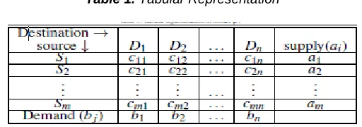
3. MODAL REPRESENTATION
In general terms, the transportation problems are related to transporting goods from m sources to n destinations with least expenses while satisfying all supply and demand limitations. The sources may be production facilities, warehouses etc and the destinations may be sales, warehouses, outlets etc. This problem is widely known as cost minimizing transportation problem. In these problems, the decision maker is sure about the transportation cost, availability and demand of the product to be transported from factories to retail stores. A cost
minimization transportation problem is formulated as:\
where
m number of sources (Si) n number of destinations (Dj) ai supply amount of the product at Si, bj demand of the product at Dj
xij amount of homogeneous product to be transported from Si to Dj
cij unit transportation cost of the product from Si to Dj ai and bj are given non-negative numbers.
Table 1. Tabular Representation
Remark 1. The above problem is said to be balanced if the total supply of the goods is same as its demand, otherwise the problem is said to be unbalanced.
4. PROPOSED ALGORITHM FOR KCM
The proposed KCM is an alternate approach for finding an IBFS for the transportation problems . This approach is based on making allocations to the minimum cost cell corresponding to row/column of maximum cost cell of TP. Our main aim to introduce this method is to minimize total transportation cost in very easy way with simple calculations. Next, Some important notations to proceed our proposed method are given.
Cost Cell (cij) : unit transportation cost of the product from Si
to Dj. Basic Cell (crs) : Maximum cij.
Basic Row Cell (crp) Minimum cost cell in corresponding row of crs.
Basic Column Cell (cts) Minimum cost cell in corresponding column of
crs
Key Cell (T) Minimun of crp and cts .
Allocation (xij) amount of homogeneous product to be
transpotated from Si to Dj
By using above notations general steps of proposed algorithm are as follows:
Step 1: Problem Representation
Represent the given transportation problem as Table 1.
Step 2: Balance the unbalanced problem
If total availability and total demand of product is equal, then go to Step 3. Otherwise balance the given problem by introducing the dummy source or destination according to the lesser availability or lesser demand, respectively.
Case 2a:
If , add a dummy source Sm+1 with availability equal to
Case 2b:
If , add a dummy destination Dn+1 with
demand equal to .
Step 3: Cell Selection and Allocation From the Transportation Problem Table
a: Choose Basic Cell.
b: Choose Basic Row Cell.
If tie occurs in selecting Basic Row Cell, then select that one, which has maximum cost cell in corresponding column.
c: Choose Basic Column Cell.
If tie occurs in selecting Basic Column Cell, then select that one, which has maximum cost cell in corresponding Row.
d: Choose Key Cell.
If basic Row and Column cell are equal, then select that one, which has maximum cost cell in corresponding column/row resp.
e: Make maximum possible Allocation to Key Cell.
f: Cross out the row/column for which supply/demand is fully satisfied.
Note: If tie not broken by using tie breakers in all above cases, then choose arbitrarily.
Step 4: Stopping Criteria
Repeat the step 3 for uncrossed row/column till all allocations are completed.
Remark 2. Make allocation in the dummy row/column at the end , when allocations are completed for all other rows and columns.
Representation of the proposed method for the balanced Transportation Problem is given by flow chart
5. NUMERICAL EXAMPLES
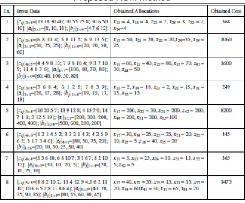
For checking the performance of proposed KCM method, theoretical work is not sufficient. So it is necessary to apply it in practical field. For this, we have applied our proposed KCM method on 12 examples taken from literature and 8 randomly generated problems , which are as given in Table 2 and Table 3 with IBFS obtained by applying proposed KCM method.
6. COMPARATIVE STUDY AND ANALYSIS
VAM is commonly used method to find initial basic feasible solution in most of transportation problems. Also, Storozhyshina et al. [36] analysed that MDM gives more efficient solution than other existing algorithms. So we have
compared the solution of our developed KCM method with solution of VAM and MDM by solving examples given in Table 2 and Table 3. For comparative study, we used modified distribution method to find optimal solution and IBFSs are obtained by applying VAM, MDM and KCM for considered examples is given in Table 4 and Table 5.
Table 2: 12 Numerical Examples taken from literature and IBFS using Proposed KCM Method
Table 4: Results(IBFS and Optimal Solution of 12 examples taken from literature)
Table 5: Results(IBFS and Optimal Solution of randomly generated 8 examples )
It can be observed from Table 4 and Table 5 that KCM obtained better initial solution than MDM for 17 examples out of 20 examples solved and for remaining 3 examples both KCM and MDM obtained same initial solution. Again KCM obtained better initial solution than VAM for 18 examples out of 20 examples solved and for remaining 2 examples both KCM and VAM gives same initial solution. Also IBFS obtained by KCM for 18 examples out of 20 examples provide optimal solution, whereas VAM provides optimal solution for only 2 and MDM provides for 3 examples. Here, we give the comparative study of our technique with VAM and MDM method with respect to optimal solution by applying ARPD technique, which is used by Mathirajan (2004). The technique is as follows:
Where ARPD(M)-Average relative percentage deviation of the given method “M”, where “M” indicates NWCM, or VAM, or LCM, or HCDM, or EDM, or TOM, or TOCM-VAM, or Proposed Method; RPD(M, K)-Relative percentage deviation of the kth problem between IBFS using method “M” and
Optimal Solution;N-the number of problems
presented;(IBFS)k-IBFS of kth problem using method M;(OS)k- optimalsolution of kth problem. By using above measures RPD and ARPD of different methods are as given in Table 6 and Table 7.
Table 6: Results related to 12 examples taken from literature (RPD and ARPD in % )
Table 7: Results related to 8 randomly generated examples (RPD and ARPD in % )
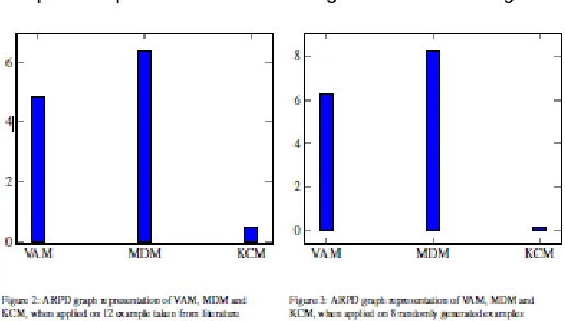
Graphical representation ARPD is given firure 2 and figure 3.
From the above graph, it can be concluded that ARPD of our proposed KCM method is least comparative to VAM and MDM, which shows the effectiveness of the proposed method. Also comparative study of number of iterations to reach optimal solution by MODI method on starting with IBFS obtained by VAM, MDM and KCM is carried out for all considered 20 examples. Results are given for each category of examples in Table 8 and Table 9.
Table 8: Results (number of iteration taken to reach optimal solution on starting with IBFS obtained by VAM, MDM and
KCM for 12 examples taken from literature)
Table 9: Results (number of iteration taken to reach optimal solution on starting with IBFS obtained by VAM, MDM and
KCM for 8 randomly generated examples)
From Table 8 and Table 9, it can be observed that KCM takes zero iterations to reach optimal solution for considered examples except for 2 examples and in these examples KCM does not take more iterations to reach optimal solution than VAM and MDM.
7. CONCLUSIONS
method, VAM and MDM with respect to optimal solution has been carried out with the help of ARPD technique. From the comparative analysis of developed KCM method with existing method, it is to be noted that KCM obtains better and effective IBFS and developed technique is very easy to apply and consume less time to compute. Also an individual can apply this technique easily to find total transportation cost of large scale TP because there is simple calculation while making allocations. The main aim of the algorithm is to avoid the transportation through the way, on which transportation cost is maximum. Because by doing this transportation cost can be minimized easily, which is the first choice of organizers. Also the present paper can be extend in future by using linear programming software for reporting obtained results as CPU times and computer memory.
References
[1]. Adlakha V, Kowalski K (1999). An alternative solution algorithm for certain transportation problems, INT. J. MATH. EDUC. SCI. TECHNOL. 30(5): 719-728. [2]. Arsham H, Kahn AB (1989). A simplex-type algorithm
for general transportation problems:An alternative to Stepping-Stone.J. Oper. Res. Soc. 400(6): 581- 590. [3]. Balakrishnan N (1990). Mdified Vogels Approximation
Method for the unbalanced transportation problem. Appl. Math. Lett. 3(2): 9- 11.
[4]. Balinski MS, Gomory RE (1964). A primal method for the Assignment and Transportation Problem. Manag. Sci. 10: 578-593.
[5]. Charnes A, Cooper WW (1954). The stepping-stone method for explaining linear programming calculations in transportation problems. Manag. Sci. 1(1): 49- 69. [6]. Dantzig GB (1951). Application of the simplex method
to a tra nsportation problem. Activity Analysis of Production and Allocation. Koopsmans TC, Ed., 359-373.
[7]. Dantzig GB (1963). Linear Programming and Extensions. Princeton, NJ:Princeton University Press. [8]. Dwyer PS (1955). The solution of the hitchcock
Transportation Problem with a method of reduced matrices. University of Michigan.
[9]. Gass SI (1990). On solving the transportation problem. J. Oper. Res. Soc. 41(4): 291- 297.
[10]. Gleyzal A (1955). An Algorithm for solving the Transportation Problem. J Res Natl Bur Stand. 54(4): 213-216
[11]. Goyal SK (1984). Improving VAM for unbalanced transportation problems. J. Oper. Res. Soc. 35(12): 1113- 1114
[12]. Goyal SK (1991). A note on a heuristic for obtaining an initial solution for transportation problem. J. Oper. Res. Soc.42(9): 819-821.
[13]. Hitchcock FL (1941). The Distribution of a product from several sources to numerous localities. J.Math. Phy. 20: 224- 230.
[14]. Ji P, Chu KF (2002). A dual matrix approach to the transportation problem. Asia Pac J Oper Res. 19(1): 35-45.
[15]. Juman ZAMS, Hoque MA (2015). An efficient heuristic to obtain a better initial feasible solution to the transportation problem. Appl Soft Comput. 34: 813-826.
[16]. Kasana HS, Kumar KD (2004). Introductory Operations Research:Theory and Applications. Springer, Heidelberg.
[17]. Khan AR (2011). A re-solution of transportation problem:an algorithmic approach. Jahangirnagar University of journal of Science. 34(2): 49- 62.
[18]. Kirca O, Satir A (1990). A heuristic for obtaining an initial solution for transportation problem. J. Oper. Res. Soc. 41(9); 865- 871.
[19]. Korukoglu S, Balli S (2011). An improved Vogels Approximation method for the transportation problem. Mathematical and Computational Applications. 16(2): 370- 381.
[20]. Koopmans, T. C. (1947). Optimum utilization of the transportation system, Econometrica, Vol. 17,pp. 3- 4. [21]. Kulkarni SS (2012) On initial basic feasible solution for transportation problem-A new approach. J. Indian Acad. Math. 34(1): 19-25.
[22]. Kulkarni SS, Datar HG (2010) On solution to modified unbalanced transportation problem. Bulletin of marathwada Mathematical Society. 11(2): 20- 26. [23]. Mathirajan M, Meenakshi B (2004) Experimental
analysis of some variants of Vogels approximation method. Asia Pac J Oper Res. 21(4): 447- 462. [24]. Pargar F, Javadian N, Ganji AP (2009). A heuristic for
obtaining an initial solution for the transportation problem with experimental analysis. The 6th International Industrial Engineering Conference, Sharif University of Technology, Tehran, Iran.
[25]. Ramakrishnan CS (1988). An improvement to Goyals modified VAM for the unbalanced transportation problems. J. Oper. Res. Soc. 39(6): 609- 610.
[26]. Rashid A (2016). Development of a simple Theorem in solving Transportation Problems. Journal of Physical Science. 21: 23-28.
[27]. Rashid A, Ahmad SS, Uddin MS (2013). Development of a new heuristic for improvement of initial basic feasible solution of a balanced transportation problem. Jahangirnagar University Journal of Mathematics and Mathematical Science. 28: 105-112. [28]. Ray GC, Hossian ME (2007). Operation Research.
First Edition, Bangladesh.
[29]. Reinfeld NV, Vogel WR (1958). Mathematical
Programming. Englewood Cliffs. New
Jersey:Prentice-Hall.
[30]. Russell EJ (1969). Extension of Dantzigs algorithm to finding an initial near-optimal basis for transportation problem. Oper. Res. 17: 187-191.
[31]. Shafaat A, Goyal SK (1988). Resolution of degeneracy in transportation problems. J. Oper. Res. Soc. 39(4): 411- 413.
[32]. Sharma JK (1989). Mathematical models in operation research. Tata McGraw Hill Publications.
[33]. Sharma RRK, Sharma KD (2000). A new dual based procedure for the transportation problem. Eur. J. Oper. Res. 122: 611-624.
[34]. Shih W (1987). Modified Stepping-stone method as a teaching aid for capacitated transportation problems. Decis. Sci. 18: 662- 676.
[36]. Storozhyshina N, Parger F, Vasko FJ (2011). A comrehensive empirical analysis of 16 heuristics for the transportation problem.OR Insight. 24(1): 63-76. [37]. Sudhakar VJ, Arunasankar N, Karpagam T (2012). A
new approach for finding an optimal solution for transportation problems. Eur. J. Sci. Res. 68(2): 254-257.
[38]. Taha HA (2006). Operation Researc: An introduction. Prentice-Hall of India.