An Efficient Radio Frequency Interference Recognition Using End-to-end Transfer Learning

Article

An Efficient Radio Frequency Interference

Recognition Using End-to-end Transfer Learning

Sahar Ujan *, Neda Navidi and Rene Jr Landry

LASSENA Laboratory, Ecole de Technologie Superieure (ETS), 1100 Notre-Dame Street West, Montreal, QC H3C 1K3, Canada; [email protected] (N.N.); [email protected] (R.J.L.) * Correspondence: [email protected]

Abstract:Radio Frequency Interference (RFI) detection and characterization has a critical role to in ensuring the security of all wireless communication networks. Advances in Machine Learning (ML) have led to the deployment of many robust techniques dealing with various types of RFI. To sidestep an unavoidable complicated feature extraction step in ML, this paper proposes an efficient end-to-end method using the latest advances in deep learning to extract the appropriate features of the RFI signal. Moreover, this study utilizes the benefits of transfer learning to determine both the type of received RFI signals and their modulation types. To this end, the scalogram of the received signals is used as the input of the pre-trained convolutional neural networks (CNN), followed by a fully-connected classifier. This study considers a digital video stream as the signal of interest (SoI), transmitted in a real-time satellite-to-ground communication using DVB-S2 standards. To create the RFI dataset, the SoI is combined with three well-known jammers namely, continuous-wave interference (CWI), multi-continuous-wave interference (MCWI), and chirp interference (CI). This study investigated four well-known pre-trained CNN architectures, namely, AlexNet, VGG-16, GoogleNet, and ResNet-18, for the feature extraction to recognize the visual RFI patterns directly from pixel images with minimal preprocessing. Moreover, the robustness of the proposed classifiers is evaluated by the data generated at different signal to noise ratios (SNR).

Keywords: Radio frequency interference detection, Deep learning, Transfer learning, Pre-trained convolutional neural networks.

1. Introduction

Recent advances in Software-Defined Radios (SDR) and cognitive networking technologies, as well as increasing the accessible low-cost hardware, have led to most applications becoming dependent on the wireless networks [1]. It provides adversaries with an opportunity to deploy the jamming attacks (also known as the intentional RFI) and harm systems that rely on wireless networks [1]. Jamming attacks cause Denial-of-Service (DoS) problems such as slowing browsing websites and downloading files, intensively limiting the number of active voice users, and as a result, network latency [2]. The jammers can be launched using simple and cheap technologies, however, they are hard to completely defeat due to the large variety of available jammers [3].

To guarantee the Quality of Service (QoS) and security of the wireless communication system, a robust RFI detection strategy is highly required to produce an effective mitigation process [3]. In addition, it is essential to precisely determine the modulation type of SoI combined by any type of RFI. Since, Automatic Modulation Classification (AMC) is a significant procedure in communication networks to facilitate the demodulation process at the receiver side [4].

To address this concern, Machine Learning (ML) based techniques have shown promising results in the area of multi-class RFI recognition [5,6] and Automatic modulation classification (AMC) [6]. However,

the complex nature of tasks like pre- processing, feature extraction, feature selection etc in classical ML techniques highly degrades the classification precision regarding efficiency and accuracy [7]. To tackle these issues, deep learning (DL) neural networks, as a subfield of ML, have presented outstanding results in the area of RFI detection. DL-based techniques include numerous information processing layers in a hierarchical design for either pattern classification or feature extraction [8]. One of the most successful types of DL is Convolutional Neural Networks (CNN) which has been typically used for object detection in computer vision fields, without any prior knowledge regarding to the object’s location [9].

The main challenge of DL in applications with supervised learning tasks could be the lack of enough dataset to train the model from the scratch. To address this issue, image-based transfer learning method has gained attraction in case of insufficient dataset to create models [10,11]. Transfer learning refers to reuse the pre-trained CNN architectures on a pre-build large dataset, such as ImageNet project [10]. Hence, transfer learning leads to minimize the training time with considering the pre-trained layers of a model [10].

In this paper, we propose a hierarchical classification design for RFI classification and AMC by leveraging the benefits of transfer learning technology using pre-trained CNNs such as AlexNet, VGG16, GoogleNet and ResNet18 for feature learning, followed by a fully-connected classifier. This study provides a comparative analysis of these pre-trained CNNs with respect to accuracy in the context of transfer learning and consumed training time. We have generated a visual representations of the received signals in time-frequency domain as the input data, which is the magnitude squared of the wavelet transform known as scalogram [12].

In this work, SoI is a video stream transmitted in a real-time digital video broadcasting scenario based on DVB-S2 standards in a Satellite communication (Satcom). We have assumed that SoI is combined with three well-known types of jammers, namely, continuous wave interference (CWI), multi-CWI (MCWI), and chirp interference (CI), to increase the scenarios complexity and to simulate the realistic situations [5]. As a result, the proposed methodology can precisely determine the type of the received signal either is SoI or a combination of SoI with any other jammers, and also the modulation type of SoI. We have investigated four different types of modulation due to their more applicable, namely, quadrature phase shift keying (QPSK), 8-array asymmetric phase-shift keying (8-APSK), 16-array APSK (16-APSK), and 32-array APSK (32-APSK).

The rest of this paper presents the related works in section 2, the proposed methodology in section 3 and the simulation results are provided in section 4. Finally, the paper is concluded in section 5.

2. Related Works

With rapid advances of AI technology, DL is also increasingly being applied to the field of RFI and modulation classification. To name a few, in [13] a robust Dl-based technique is proposed known as faster region-based convolutional neural networks (Faster R-CNN) for interference and clutter detections in a high-frequency surface wave radar (HFSWR). To this end, the Range-Doppler (RD) spectrum image is used as the input of the designed network. As the results , the proposed method has a high classification accuracy and a decent detection performance [13].

Z. Yang and et. al, have proposed a CNN-based strategy named RFI-Net to detect interference in a five-hundred-meter Aperture Spherical radio Tele-scope (FAST) [14], that can outperform other techniques such as the U-Net model based on a CNN architecture, k-nearest neighbors (KNN) algorithms, as well as Sum-Threshold. In [15], two DL-based strategies are used for jamming attack detection, namely deep convolutional neural networks (DCNN) and deep recurrent neural networks (DRNN). In this research, two different jamming attacks, namely, classical wide-band barrage jamming and reference signal jamming have been analyzed [15]. The results show that the classification accuracy reaches up to 86.1% under a realistic test environment [15].

proposed to recognize ten different modulation types. The results show the classification accuracy is increased up to 90% at high SNRs. Further Principal Component Analysis (PCA) has been deployed to optimize the classification process by minimizing the size of training dataset [16]. A combination of the transfer learning and a pre-trained Inception-ResNetV2 has been presented in [17] to recognize three modulation types namely Binary Phase Shift Keying (BPSK), QPSK and 8PSK at SNR equal to 4 dB. As the results indicate, the classification accuracies to recognize BPSK, QPSK and 8PSK are 100%, 99.66% and 96.33% respectively [17].

In [18], a robust hierarchical DNN architecture is presented that performs a hierarchical classification to estimate data type (Analog or digital modulation), modulation class, and modulation order. To this purpose, spectrogram snapshots computed from baseband In-phase and Quadratic ( I/Q ) components of the signal are used as the input of the CNN and reach out the performance of 90% at high SNR for most modulation schemes [18]. Yang et al. present an efficient methodology using CNN and recurrent neural networks (RNN) to classify six modulation types under two channel distortions such as Additive White Gaussian noise (AWGN) and Rayleigh fading [19]. According to the experimental results, the classification precision of the CNN is always close to 100% in AWGN channel [19]. Even in Rayleigh channel, the minimum classification accuracy still approaches to 84%, whereas the maximum value is near to 96%. [20] proposes a robust CNN-based approach which can precisely classify four types of modulation including BPSK, QPSK, 8PSK, and 16QAM in an orthogonal frequency division multiplexing (OFDM) system under presence of Phase offset (PO). In [21], CNN and LSTM have been used to solve AMC problem. Furthermore, the proposed classifiers based on the fusion model in serial and parallel modes are of great benefit to improving classification accuracy when the SNR is ranging from 0 dB to 20 dB [21]. As is shown, the serial fusion mode has the best performance compared with other modes. As it was already mentioned, in our study a transfer learning-based approach is proposed for RFI recognition and AMC.

3. Proposed Methodology

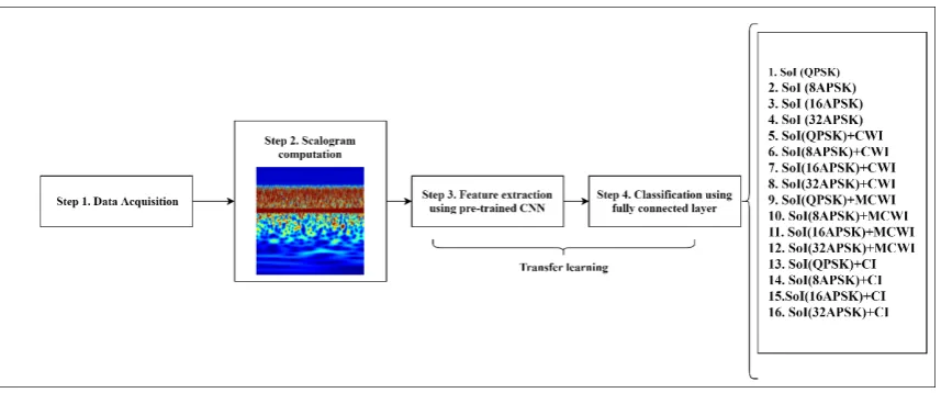
This study proposes a DL-based approach for RFI recognition and AMC by benefiting from transfer learning strategy. The general framework is based on the hierarchical classification proposed in [6], which the first and second levels determine the type of the received signal that is either SoI or a combination of SoI with any of the jamming signals and the modulation type of SoI, respectively. To this end, in the first classification level, a classifier is trained to determine the type of the received signals. Further, a classifier is trained per each type of received signal to recognize the modulation type. Figure 1demonstrates the proposed methodology, which follows four steps: 1) data acquisition, 2) wavelet coefficients scalograms calculations, 3) Feature extraction using pre-trained CNN, and 4) classification. Each step will be fully elaborated in the rest of this section.

3.1. Data acquisition set-up

As fully explained in [5,6], the desired signal is a real-time video stream, which is modulated and processed by GNU radio and transmitted using a Universal Software Radio Peripheral (USRP-N210) [22]. For modeling a real-time Satcom channel simulator (RTLogic T400) [23] is used. Further, the generated jamming signals are combined to SoI by a combiner. Finally, the combined signal is received by a MegaBee modem [5]. Notably, AWGN power can be manually adjusted in the range of -168 to -125 dBm which is approximately equal to SNR 5 to 12 dB. Figure 2shows the Real-time RFI data

acquisition set-up.

Figure 2.Real-time RFI data acquisition set-up Table 1presents a summary of the dataset specification generated in [5].

Table 1.Real-time dataset specification.

Characteristic Value

Total number of observations 4800

Length of each generated signal 32448 (8 ms)

Sampling frequency 40x106Hz

Modulation types QPSK, 8APSK, 16APSK, and 32APSK

AWGN power 140dBm(SNR∼=9dB)

No. of each class of signals per modulation type 300

This study analyzes the efficiency of the proposed classification technique in the presence of three jamming signals, such as, continuous-wave interference (CWI), multi-CWI (MCWI), and chirp interference (CI) [5].

1) Continuous Wave Interference (CWI):

CW=exp(j2πfcwt) (1)

Where fcwandtrepresent the center frequency and the duration of interference respectively.

2) Multi Continuous Wave Interference (MCWI):In this study, we have considered two-tone CW which is defined as:

MCW=exp(j2πfc₁t) +exp(j2πfc2t) (2) Where fc1 and fc2are the center frequencies of each wave.

3) Chirp Interference (CI):The CI has been generated according to [24] as follows:

Chirp=exp(2πk 2t

2₊₂

wherek= f1−f0

T so that the signal sweeps fromf0to f1andTis the sweeping duration.

Note: the center frequencies have been considered to be changed randomly.

3.1.1. Dataset generation

This study has considered visual representation of the received signals in time-frequency domain using scalogram as an input data. Scalogram is the squared magnitude of Continuous Wavelet Transform (CWT) and mathematically is defined as[25]:

zx(α,τ) =|√1

α Z +∞

−∞ x(t)Φ

∗₍t−τ α )dt)|

2 ₍₄₎

where,zandΦ∗denotes scalogram and complex conjugate of the mother wavelet function.αand τare the oscillatory frequency and shifting position of the wavelet, respectively [25]. CWT is widely applied for non-stationary and transient signal analysis, mainly through its scalogram [26]. The main difference between wavelet transform and short-time Fourier transform (STFT) is that STFT has a fixed signal analysis window whereas the wavelet transform utilizes short windows at high frequencies and long windows at low frequencies [12].

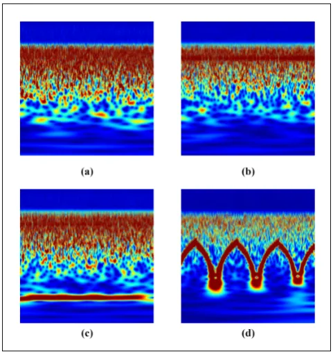
Therefore, the wavelet transform provides superior time and frequency resolution at high and low frequencies respectively [12]. Hence, the wavelet-based analysis is considered as an appropriate choice when the signal at hand has high frequency components for short duration and low frequency components for longer durations which are considered in this study [12]. As shown in Figure 3, scalograms of SOI and its combination with CWI, CI and MCWI samples are computed using the Morse wavelet [27]to calculate the wavelet transform as well as the coherence analysis of the time series, and has been converted to an RGB image.

Figure 3.Scalogram representation of target classes: a) SoI, b) SoI+CWI, c) SoI+MCWI, and d) SoI+CI

3.2. Transfer learning process

higher level features so the layer right before the classification phase can be a good choice for feature extraction [30].

A typical CNN structure consists of two parts; 1) convolutional layers, composed by a stack of the convolutional and the pooling layers to extract the features from the image-based input. 2) a classification part including a set of fully-connected (FC) layers followed by an activation function, like Soft-Max, to classify the images using the extracted features [11]. In the transfer learning process, the classification part can be replaced by a new classifier which fits to the objective of the application. The model can be tuned using one of the following strategies [11]:

• Training the entire data-set: The pre-trained CNN can be trained from the scratch using a new dataset. Therefore, a large dataset and lots of computational power are required.

• Training some layers and leaving the others frozen: As the lower layers extract the general features while higher layers represent the most specific features, it can be decided how many of layers needs to be re-trained depending on the objective of the application. For a small dataset with a large number of parameters, it is efficient to leave more layers frozen. The frozen layers are kept unchanged during the training process to avoid the overfitting. On the other hand, for a large dataset with a small number of parameters, training more layers would be reasonable to the new task, since overfitting is not an issue.

• Freezing the convolutional part: in this scenario the convolutional part can be kept unchanged and its output can be fed to a new classifier. In the other words, the pre-trained models are considered as a fixed feature extraction basis which is beneficial in case of having a small dataset and suffering from lack of computational power. Notably, in this study, we have applied this strategy.

It should be taken into account that the first two strategies highly depend on the learning rate hyper-parameter which defines how much the weights of a network can be adjusted. Small value learning rate can be chosen over high value learning rate to reduce the risk of losing previous knowledge [11]. We present pre-trained CNNs and fully connected classification in the following sections.

3.2.1. Pre-trained CNNs

As it is presented in the previous section, transfer learning refers to reuse of pre-trained CNN architectures on a large dataset. In this study, we have analyzed the efficiency of four well-known CNN architectures, namely, AlexNet [9], GoogleNet [31], ResNet18 [32] and VGG16 [33] regarding to classification precision and training time, as you can see below:

• AlexNet: In 2012, AlexNet could outperform other prior architectures in ImageNet LSVRC-2012 competition, designed by the SuperVision group [9]. AlexNet includes five convolutional layers and three FC layers in which Relu is applied after every convolutional and FC layer. Also dropout technique is applied before the first and the second FC layer [9].

• GoogleNet : GoogleNet won ILSVRC 2014 competition with a high precision close to human’s perception. Its architecture has taken benefits of several small convolutions in order to drastically reduce the number of parameter. It consists of a 22 layer deep CNN but reduced the number of parameters from 60 million (AlexNet) to 4 million [31].

• ResNet: Residual Neural Network (ResNet) presented an outstanding performance in ILSRVC 2015 [32]. The Residual network directly copies the input matrix to the second transformation output and sums the output in final ReLU function [32].

It should be taken into account that output of the following layers has been used as the feature set for the designed classification; “fc8” for AlexNet and VGG16, “loss3-classifier” and “fc1000” for GoogleNet and ResNet18 respectively. Since, these are the last layers of the convolutional structure before the classification layer. Notably, the input image size for AlexNet is 227 by 227 and 224 by 224 for the three other CNNs.

3.2.2. Fully Connected (FC) layer

In CNN, the convolutional and pooling layers can be followed by a set of FC layers that performs like any ANN such as MLP. The purpose of the FC layers is to combine all the features (local information) learned by the previous layers across to recognize the larger patterns. For classification problems, the number of neurons at the last FC layer is equal to the number of classes [34]. In image classification problems, the standard method is to use a stack of FC layers, followed by a Soft-Max activation function [11]. The output of Soft-Max is a set of probability distributions of different classes, and where the neuron with the maximum probability is considered as the classification result [35]:

Plabel =

exp(f ormer layer output)

∑k

i=1(f ormer layer output)

(5)

where,Ppresents the prediction, the former layer output refers to the last fully connected layer, and k represents the number of fully connected layers. The fundamental of the training phase is like MLP that after defining the CNN layers, the training phase is started by determining the optimization technique first. There are two well-known optimizers to minimize the loss function (Eq. 6), such as adaptive moment estimation and Stochastic Gradient Descent (SGD) [36]. In this research, the loss function is the cross-entropy which is mathematically defined as:

loss=

N

∑

i=1

K

∑

j=1

tijlnPlabelij (6)

where,NandKrefer to number of samples and classes respectively. tijis an indicator thatith

sample belongs tojthclass [36]. 4. Results and Discussion

In this section, we illustrate the simulation results of the proposed methodology for both RFI recognition and AMC, using MATLAB. We evaluate the performance of the four pre-trained CNNs (AlexNet, GoogleNet, VGG 16 and ResNet18) to classify the received signal and the modulation type. The results show a comparative analysis of these pre-trained CNNs with respect to the accuracy in the context of transfer learning and consumed training time. The architecture of the FC part for each classifier includes a layer with four neurons, followed by a Soft-Max classifier. In the experiments, the highest classification results are achieved using SGD with momentum (SGDM) and Adam optimizers for the RFI classification and AMC phases, respectively.

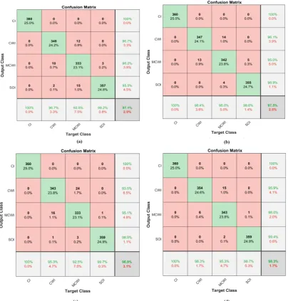
4.1. Simulation results for RFI classification

Figure 4.RFI classification phase results using a) AlexNet (97.1%), b) VGG16 (97.5%), c) GoogleNet (96.9%) and d) ResNet18 (98.3%)

Figure 5illustrates a comparative result of the elapsed running time using each pre-trained CNN architecture. The consumed time has been computed using “tic-toc” function of MATLAB. It is clear that AlexNet is comparatively less time-consuming and more efficient.

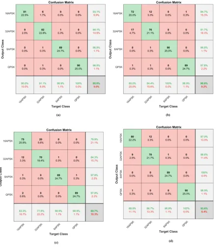
4.2. Simulation results of AMC

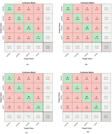
For the AMC phase, we have trained another classifier per each received type of signal to specify the modulation type of the received signals. Notably, the SoI is transmitted using four modulation types: QPSK, 8APSK, 16APSK, and 32APSK. The following figures illustrate the AMC results for each received signal. As can be seen, the presence of jammers highly degrades the classification accuracy. As Figure 6indicates that AMC is more efficient using AlexNet in the absence of jamming signals, with a comparative classification precision of 95.00%.

Figure 6.AMC result in the presence of SoI (AMC1) using (a) AlexNet (95%), (b) VGG16 (90.08%), (c) GoogleNet (89.7%), and (d) ResNet18 (93.6%)

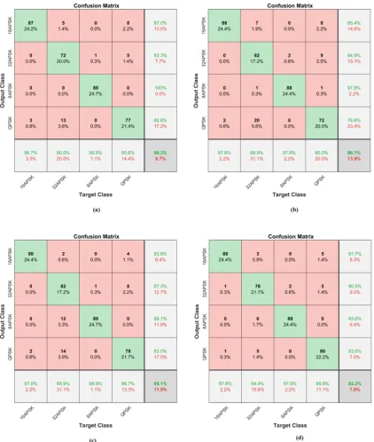
Figure 7.AMC results in the presence of CWI (AMC2) using a) AlexNet (90.30%), VGG16 (86.1%), GoogleNet (88.1%) and ResNet18 (92.2%)

Figure 8.AMC results in the presence of MCWI (AMC3) using a) AlexNet (71.4%), b)VGG16 (71.9%), c) GoogleNet (71.10 %) and d) ResNet18 (71.7%)

Figure 9.AMC results in the presence of CI (AMC4) using a) AlexNet (79.20%), b) VGG16 (87.30%), c) GoogleNet (78.10%) and d) ResNet18 (81.90%)

According to the AMC results, ResNet18 is more efficient because it shows a higher average accuracy comparatively.

4.3. Prediction phase

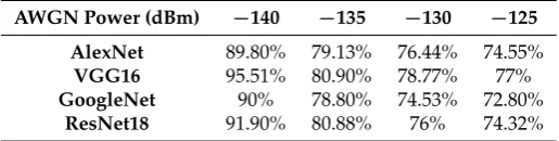
Table 2.prediction results of the trained CNNs for RFI classification at different noise powers

AWGN Power (dBm) −140 −135 −130 −125

AlexNet 89.80% 79.13% 76.44% 74.55%

VGG16 95.51% 80.90% 78.77% 77%

GoogleNet 90% 78.80% 74.53% 72.80% ResNet18 91.90% 80.88% 76% 74.32%

According to the results, VGG16 shows a more precise performance in detecting the type of unseen RFI at different noise levels.

Tables3–6illustrate the prediction results for each AMC (SoI, SoI+CWI, SoI+MCWI and SoI+CI ) using the trained classifiers using different pre-trained CNNs

Table 3.The prediction result for AMC1

AWGN Power (dBm) −140 −135 −130 −125

AlexNet 94% 84% 52% 45.50%

VGG16 85.50% 53% 48.70% 42.25%

GoogleNet 87% 56.25% 38.25% 36.50% ResNet18 92.41% 56.25% 42.25% 40.70%

As it was shown, in the absence of jamming signals, AlexNet performs more efficiently to recognize the modulation types in different noise powers.

Table 4.The prediction result for AMC2

AWGN Power (dBm) −140 −135 −130 −125

AlexNet 90.03% 58.50% 40% 37.50%

VGG16 85.83% 52% 41% 31.50%

GoogleNet 87.88% 55.60% 44.13% 39.50%

ResNet18 91.03% 69% 50% 40.50%

As Table 4shows, ResNet18 performs more accurately compared to the other classifiers.

Table 5.The prediction result for AMC3

AWGN Power (dBm) −140 −135 −130 −125

AlexNet 70.25% 58.50% 31.50% 24.90%

VGG16 71.91% 69.50% 50.50% 40%

GoogleNet 67.50% 62% 41% 31%

ResNet18 70.91% 64% 45% 37%

In the presence of MCWI, VGG16 is more robust in recognizing four different modulation types.

Table 6.The prediction result for AMC4

AWGN Power (dBm) −140 −135 −130 −125

AlexNet 78.60% 55% 52% 45%

VGG16 77% 56% 53% 44%

GoogleNet 76.70% 56.50% 50.50% 43%

ResNet18 80% 59.50% 58% 47%

depending on type of data. To sum up, ResNet-18 shows more promising results. However, the presented techniques are highly sensitive to AWGN power. As is shown, the classifiers are less reliable by increasing the AWGN power.

5. Conclusions

In this work, we presented a transfer learning-based approach for RFI recognition and modulation classification. In this approach, the pre-trained CNN analyzes the scalogram of the received signal to extract more informative features which will be further used in the classification phase using fully-connected layer followed by a soft-max activation function. This work presented a comparative analysis of using four well-known pre-trained CNNs such as AlexNet, GoogleNet, VGG16 and ResNet18. As this results show, the classification accuracy highly depends on the type of the input data. More importantly, the dataset used as the input in this study includes the scalogram of the signals transmitted in a satellite-to-ground video broadcasting scenario based on DVB-S2 standards. Further, the robustness of each trained classifier in predicting unseen data was fully evaluated. To sum up, in terms of classification, all the pre-trained architectures perform relatively similarly, although AlexNet and VGG16 have the least and the most elapsed training times.

6. Materials

The generated dataset in this study is available athttps://doi.org/10.5281/zenodo.3958266. This dataset includes the scalogram of the RFI signals in four modulation type including QPSK, 8APSK, 16APSK and 32APSK.

Author Contributions:The overall study supervised by R.J.L.; Methodology, Software and preparing the original draft by S.U.; review and editing by N.N.; The results were analyzed and validated by R.J.L. All authors have read and agreed to the published version of the manuscript.

Funding:This research is part of the project entitled AVIO-601 in LASSENA Lab (École de Technologie Supérieure) named Interference Mitigation in Satellite Communication. It is supported by the Natural Sciences and Engineering Research Council of Canada (NSERC), Thales, Telesat, VIGILANT GLOBAL, CRIAQ, and Atem Canada.

Acknowledgments:Special thanks to CMC for providing the required equipment to succeed with this project

Conflicts of Interest:The authors declare no conflict of interest.

References

1. S. Weerasinghe; T. Alpcan; S. M. Erfani; C. Leckie; P. Pourbeik; and J. Riddle, Deep learning based game-theoretical approach to evade jamming attacks,in International Conference on Decision and Game Theory for Security, 2018: Springerpp. 386-397.

2. J. Geier. Wireless LAN Implications, Problems, and Solutions,http://www.ciscopress.com/articles/article. asp?p=2351131&seqNum=2[accessed 10 Feb, 2020].

3. K. Grover, A. Lim, and Q. Yang, Jamming and anti-jamming techniques in wireless networks: a survey, International Journal of Ad Hoc and Ubiquitous Computing, vol. 17, no. 4, pp. 197-215, 2014.

4. O. A. Dobre, A. Abdi, Y. Bar-Ness, and W. Su, Survey of automatic modulation classification techniques: classical approaches and new trends, IET communications, vol. 1, no. 2, pp. 137-156, 2007.

5. Ujan, S.; M. H. S. Rene Jr Landry, A Robust Jamming Signal Classification and Detection Approach Based on Multi-Layer Perceptron Neural Network, International Journal of Research Studies in Computer Science and Engineering (IJRSCSE), vol. 7, no. 1, pp. 1-12, 2020 2020, doi:http://dx.doi.org/10.20431/2349-4859.0701001. www.arcjournals.org.

6. Ujan, S.; N. N. a. R. J. L., Hierarchical Classification Method for Radio Frequency Interference Recognition and Characterization, Applied Science, 2020, doi:10.20944/preprints202005.0356.v1

8. A. A. A. Lateef, S. Al-Janabi, and B. Al-Khateeb, Survey on intrusion detection systems based on deep learning, Periodicals of Engineering and Natural Sciences, vol. 7, no. 3, pp. 1074-1095, 2019.

9. A. Krizhevsky, I. Sutskever, and G. E. Hinton, Imagenet classification with deep convolutional neural networks, in Advances in neural information processing systems, 2012, pp. 1097-1105.

10. M. T. Hagos and S. Kant, Transfer Learning based Detection of Diabetic Retinopathy from Small Dataset, arXiv preprint arXiv:1905.07203, 2019.

11. P. Marcelino. Transfer learning from pre-trained models. Towards data science.https://towardsdatascience. com/transfer-learning-from-pre-trained-models-f2393f124751[accessed 15, Jan, 2020].

12. D. L. Stevens and S. A. Schuckers, Low probability of intercept frequency hopping signal characterization comparison using the spectrogram and the scalogram, Global Journal of Research in Engineering, 2016. 13. L. Zhang, W. You, Q. Wu, S. Qi, and Y. Ji, Deep learning-based automatic clutter/interference detection for

HFSWR, Remote Sensing, vol. 10, no. 10, p. 1517, 2018.

14. Z. Yang, C. Yu, J. Xiao, and B. Zhang, Deep residual detection of radio frequency interference for FAST, Monthly Notices of the Royal Astronomical Society, vol. 492, no. 1, pp. 1421-1431, 2020.

15. S. Gecgel, C. Goztepe, and G. K. Kurt, Jammer detection based on artificial neural networks: A measurement study, in Proceedings of the ACM Workshop on Wireless Security and Machine Learning, 2019, pp. 43-48. 16. S. Ramjee, S. Ju, D. Yang, X. Liu, A. E. Gamal, and Y. C. Eldar, Fast deep learning for automatic modulation

classification, arXiv preprint arXiv:1901.05850, 2019.

17. K. Jiang, J. Zhang, H. Wu, A. Wang, and Y. Iwahori, A Novel Digital Modulation Recognition Algorithm Based on Deep Convolutional Neural Network, Applied Sciences, vol. 10, no. 3, p. 1166, 2020.

18. K. Karra, S. Kuzdeba, and J. Petersen, Modulation recognition using hierarchical deep neural networks, in 2017 IEEE International Symposium on Dynamic Spectrum Access Networks (DySPAN), 2017: IEEE, pp. 1-3. 19. C. Yang, Z. He, Y. Peng, Y. Wang, and J. Yang, Deep Learning Aided Method for Automatic Modulation

Recognition, IEEE Access, vol. 7, pp. 109063-109068, 2019.

20. J. Shi, S. Hong, C. Cai, Y. Wang, H. Huang, and G. Gui, Deep Learning-Based Automatic Modulation Recognition Method in the Presence of Phase Offset, IEEE Access, vol. 8, pp. 42841-42847, 2020.

21. D. Zhang et al., Automatic modulation classification based on deep learning for unmanned aerial vehicles, Sensors, vol. 18, no. 3, p. 924, 2018.

22. National Instruments. "USRP N210 Kit."http://www.ettus.com/all-products/un210-kit/[accessed 15, Jan, 2020].

23. K. D. S. Solutions. T400CS Channel Simulator http://www.rtlogic.com/products/rf-link-monitoring-and-protection-products/t400cs-channel-simulator[accessed Aug 28, 2019].

24. T.Smyth, CMPT 468:Frequency Modulation (FM) Synthesis," Simon Fraser University„ School of Computing Science,2013.

25. Y. Yuan, G. Xun, K. Jia, and A. Zhang, A multi-context learning approach for EEG epileptic seizure detection BMC systems biology, vol. 12, no. 6, p. 107, 2018.

26. G. Lenoir and M. Crucifix, A general theory on frequency and time–frequency analysis of irregularly sampled time series based on projection methods–Part 1: Frequency analysis, Nonlinear Processes in Geophysics, vol. 25, no. 1, p. 145, 2018.

27. J. M. Lilly and S. C. Olhede, Generalized Morse wavelets as a superfamily of analytic wavelets, IEEE Transactions on Signal Processing, vol. 60, no. 11, pp. 6036-6041, 2012.

28. J. Pan and Q. Yang, Feature-based transfer learning with real-world applications, Hong Kong University of Science and Technology, 2010.

29. V. C. Raykar, B. Krishnapuram, J. Bi, M. Dundar, and R. B. Rao, Bayesian multiple instance learning: automatic feature selection and inductive transfer, in Proceedings of the 25th international conference on Machine learning, 2008, pp. 808-815.

30. MathWorks. Image Category Classification Using Deep Learning.https://www.mathworks.com/help/ vision/examples/image-category-classification-using-deep-learning.html[accessed 25 March, 2020]. 31. C. Szegedy et al., Going deeper with convolutions, in Proceedings of the IEEE conference on computer vision

and pattern recognition, 2015, pp. 1-9.

33. K. Simonyan and A. Zisserman, Very deep convolutional networks for large-scale image recognition, arXiv preprint arXiv:1409.1556, 2014.

34. MathWorks, convolution2dLayer,https://www.mathworks.com/help/deeplearning/ref/nnet.cnn.layer. convolution2dlayer.html[accessed 15, Jan, 2020].

35. H. Pokharna. The best explanation of Convolutional Neural Networks on the Internet!" https://medium.com/technologymadeeasy/the-best-explanation-of-convolutional-neural-networks-on-the-internet-fbb8b1ad5df8[accessed 15, Jan, 2020].

36. S. Reddy, K. T. Reddy, and V. ValliKumari, Optimization of Deep Learning Using Various Optimizers, Loss Functions and Dropout, Int. J. Recent Technol. Eng, vol. 7, pp. 448-455, 2018.

c