Graphical Diagnostic for Mortality Data Modeling
M.L. Gamiz∗,†, M.D. Martinez-Miranda†and R. Raya-Miranda†
Department of Statistics and O.R., University of Granada, 18010 Granada, Spain; [email protected] (M.D.M.-M.); [email protected] (R.R.-M.)
* Correspondence: [email protected]
† These authors contributed equally to this work.
Abstract: The main contribution of this paper is to develop a graphical tool to evaluate the suitability of a candidate parametric model to fit a data set. The practical motivation is to check the adequacy of the so called SAINT model proposed in Jarner and Kryger (2011). This model has been implemented in practice by an important European pension fund concerned with setting annuity reserves for all current or former employees of Denmark. So, one particular relevant question is whether this mortality model is actually fitting old-age. Our graphical test can be described as follows. First we transform the data by means of the parametric model which is being evaluated. Should the model be correct, the transformed data will be in accordance with an Exponential distribution with rate 1. Then we construct a family of local linear hazard estimates based on the data on the transformed scale. Finally we use the statistical tool SiZer to assess the goodness-of-fit of the Exponential distribution to the data on the transformed scale. If the model is correct the SiZer map should not reveal any significant feature in the family of kernel estimates. Our method allow us to establish a diagnostic regarding the validity of the SAINT model when describing mortality patterns in four different countries.
Keywords:SAINT model; SiZer; local linear fitting; mortality data
0. Introduction
The main contribution of this paper is to develop a graphical tool to evaluate the suitability of a candidate parametric model to fit a data set. The practical motivation is to check the adequacy of the so called SAINT model proposed in Jarner and Kryger (2011). This model has been implemented in practice by an important European pension fund concerned with setting annuity reserves for all current or former employees of Denmark. So, one particular relevant question is whether this mortality model is actually fitting old-age.
The SAINT model has been evaluated previously in Spreeuw, Nielsen and Jarner (2013), where a visual inspection technique is introduced in order to detect the credibility of the parametric assumptions of the proposed model. The technique consists of first transforming the original mortality data according to the proposed parametric hazard model, and then non parametrically estimate the density based on transformed data. The density of the transformed data should be close to the uniform distribution when the model assumptions are correct. To estimate the density on the transformed axis the local linear density estimator based on filtered data and proposed in Nielsen, Tanggaard and Jones (2009) is used.
1. Mixed hazard model for mortality data
1.1. Model specifications
The parametric model for mortality data suggested in Jarner and Kryger (2011), SAINT model is a multiplicative frailty model where the mortality rate of a individual is decomposed in two factors: one is a standard intensity function and the other is a non-negative random variable, the frailty. In Spreeuwet al.(2013) this model is evaluated. The authors discuss the adequacy of several candidates for the frailty variable, a Gamma model, an Inverse Gaussian model, and degenerate (i.e. no frailty) to properly adjust hazard rates based on mortality data. In their study the authors introduce a visual test to assess the validity of the mixed model to explain mortality rates based on data concerning female population of ages ranging from 40 onwards and coming from four different countries, i.e., United States, United Kingdom, Denmark and Iceland, during the year 2006. In their conclusions, the authors argue that the Gamma frailty model provides a more accurate fit to the data in all real cases considered, specially at the oldest old-ages for which the Gamma frailty model better accommodate to the presence of an old-age mortality plateau. The parametric mixed mortality model considered generalizes the classical Gompertz survival model by including more parameters and by including a multiplicative frailty component.
Specifically, the frailty model presented in Jarner and Kryger (2011) and Spreeuwet al.(2013) introduces the individual effect for life’s mortality multiplicatively. So, it is assumed that the individual effect for a particular subject is described by a random variableX, in the sense that the conditional mortality hazard at aget, givenX=x, is expressed as
α(t,x) =xα0(t), (1)
whereα0(t)represents the baseline mortality hazard at age t, that is, the hazard corresponding to an individual with frailty level x = 1. Also, it is assumed that, given a cohort of n individuals, X1,X2, . . . ,Xnare independent and identically distributed with mean 1.
We adopt here the specifications given in Jarner and Kryger (2011) for national and international mortality modeling, later analyzed in Spreeuwet al. (2013), which consist of defining the baseline mortality hazard as
α0(t) =exp
a0+a1t+a2t2
. (2)
Also, following the recommendation of Spreeuwet al. (2003) we consider for the frailtyXa gamma distribution with mean 1 and varianceσ2.
From Equation (1), the relationship between the corresponding survival functions can be written asSx(t) = e−Λx(t) = e−xΛ0(t), whereΛx(t) = Rt
0αx(s)dsis the cumulative hazard mortality for an individual for which X = x and Λ0(t) = R0tα0(s)dsis the baseline cumulative hazard. Then the cohort survival function is given by
S(t) = Z
Sx(t)f(x)dx= Z
e−xΛ0(t)f(x)dx, or, equivalently,
S(t) =LX(Λ0(t)), where, LX(s) = E
e−sX
denotes the Laplace transform of the distribution of the frailty random variable,X. From here we can express the frailty model as
α(t) =−
dlnLX(s) ds
Λ0(t)
Considering (2) and that X has a gamma distribution as stated above, LX(s) = E e−sX
=
1+σ2s−1/σ 2
, we have that the SAINT model specifies the cohort mortality hazard as
α(t) = α0(t)
1+σ2Λ0(t)
= exp a0+a1t+a2t 2
1+σ2
Rt
0exp(a0+a1s+a2s2)ds
(4)
1.2. Maximum likelihood estimation of the parametric model
Consider a data set consisting of mortality statistics ofnlives. More specifically, the information we register is related, on the one hand to the exposure processYi, which takes value 1 when individual iis alive and under observation, and, on the other hand, Ni, the counting process taking the value 1 when the individualihas died while under observation and 0, otherwise. We consider bothYiandNi depending on the aget, in such a way that we assume thatNiis a one-dimensional counting process with respect to an increasing right continuous complete filtrationFt,t>0. Also we assume that the corresponding intensity function of Ni satisfies the multiplicative model of Aalen (see for example Andersenet al., 1993)
λi(t) =α(t)Yi(t),
where, as in Spreeuw et al. (2013), we consider that{αθ,θ∈Θ}is a parametric family of hazard
functions to which the true hazard functionα = αθ belongs. In other words, the exact mortality is determined except for the value of the parameter vectorθwhich is estimated by maximum-likelihood
methods, that is,bθ=arg max θ∈Θ
L(θ), with
L(θ) =
n
∑
i=1 Zlog(αθ(t))dNi(t)− n
∑
i=1 Zαθ(t)Yi(t)dt
1.3. Transformation of data
In this section we use the parametric fit explained in the previous section to transform the data in such a way that the underlying hazard would become constant in case the parametric fit indeed would have been the correct underlying model α. The parametric fit is in other words used as a
kind of prior knowledge to simplify the non-parametric estimation problem. If the prior knowledge is of high quality and the parametric model has good approximation properties, then the resulting non-parametric problem is simplified in the second step compared to a fully non parametric treatment of the original dataset (not transformed). Next a local linear hazard estimator is applied to the transformed data. If the parametric specification αθ were true then after the time transformation
x=Λθ(t)withΛθ(t) = Rt
0αθ(s)ds, the functional form of the hazard on the transformed scale would be simply equal to the standard Exponential, i.e. the hazard would be equal to 1 on the transformed scale.
For a givenθ∈ Θwe putNeiθ = Ni◦Λ−1θ andYeiθ =Yi◦Λ−1
θ . This transformed process follows Aalen’s multiplicative hazard model with transformed stochastic hazard
λθi(x) =gθ(x)×Yi
Λ−1
θ (x)
where gθ(x) = α Λ−1 θ (x) /αθ Λ−1 θ (x)
produce a sample from an Exponential distribution with rate 1. In other words the estimated curve
b
gθshould be very close to the liney=1.
2. Local linear estimation with aggregated data
In this section we present a local linear estimation method for aggregated survival data which is based on a least squares minimization problem. We follow the general formulation proposed in Nielsen and Tanggaard (2001) and we obtain an estimator for the hazard function as well as for its first derivative. Also we derive an expression for the variance of the estimator of the derivative of the hazard function needed to develop the SiZer tool. The details are given in the following. We observe nindividualsi = 1, . . . ,n. Let Ni count observed failures for theith individual in the time interval [0,T]. Ni can take values 0 or 1. We assume that Ni is a one-dimensional counting process with respect of an increasing, right continuous, complete filtrationFt,t∈ [0,T], i.e. it obeysles conditions habituelles. We assume Aalen’s multiplicative model where the random intensity is written as
λi(t) =α(t)Yi(t), (5)
with no restriction on the functional form of the hazard functionα(·). Yi is a predictable process taking values in{0, 1}, indicating (by the value 1) when theith individual is at risk. We assume that(N1,Y1), . . . ,(Nn,Yn) are i.i.d. for the n individuals. Note that this formulation contains the important particular case of a longitudinal study with left truncation and right censoring. In that case we observe triplets(Li,Zi,δi)(i=1, ..,n) whereLiis the time an individual enters the study,Zi is the time he/she leaves the study andδi is binary and equal to 1 if death is the reason for leaving the study (censoring indicator). Then, the processYi above would beYi(t) = I[Li ≤ t < Zi] and Ni(t) = I[Zi ≤ t]δi, where I(·) is the indicator function. Hereafter we will work in the general model. Expressions for particular sampling schemes such as left truncation and right censoring can be derived just by substituting the particular expressions of the processes.
The data that we will use are divided into discrete numbers of occurrences and exposures. We suppose that the following aggregated values of occurrences and exposures are available
Or = n
∑
i=1Z xr xr−1
dNi(x), and Er = n
∑
i=1Z xr xr−1
Yi(x)dx,
for r = 1, . . . ,m. Here, x1, . . . ,xm are some time points. For simplicity in the formulation of the problem we consider this points equidistant however we can easily generalize for the non equidistant case. With∆r =xr−xr−1we can defineYr =Er/∆r. This is the average number of individuals which are at risk in the interval[xr−1,xr)forr=1, . . . ,mand withx0=0.
In this situation, we define an empirical (naive) estimator ofαras
b
αr = Or
Er.
From theorem A.1 (i) and (ii) in Wang, Muller and Capra (1998) it can be deduced (see also Bagkavos, 2011) that
E(bαr)≈α(xr),
and
Var(bαr)≈ α(xr)
S(xr) (6)
Moreover, the pairs(xr,bαr),r=1, 2, . . . ,Mcan be considered approximately independent. Under a local linear approach we assume that, for eachxr, the hazard functionαcan be locally
approximated (in a neighborhood of xr) by a linear function, this is, for all x ∈ (xr−h,xr+h),
an estimation of the interceptθ0would provide an estimation ofα(xr), whereas an estimation of the
slopeθ1would provide an estimation of the derivativeα0(xr).
To this goal, we formulate the following least squares problem
b
θ0
b
θ1
!
=arg min
θ0 θ1 M
∑
m=0(bαm−θ0−θ1(xm−xr)) 2K
h(xm−xr),
wherebαm= Om
Em.
The solution to the equations above is easy to obtain and can be expressed as
• The hazard function,α
bαLL(x) =
S2(x)T0(x)−S1(x)T1(x) S2(x)S0(x)−(S1(x))2
(7)
• The first derivative of the hazard function,α0
b
α0LL(x) =
S0(x)T1(x)−S1(x)T0(x) S2(x)S0(x)−(S1(x))2
(8)
where, as usual, we define the momentsSj, forj=0, 1, 2,
Sj(x) = M
∑
m=0(xm−x)jKh(xm−x),
and, forj=0, 1, we denote
Tj(x) = M
∑
m=0(xm−x)jKh(xm−x)bαm,
beingbαm= Om
Em, form=1, . . . ,M, andKh(·) = 1 hK
· h
, withKa symmetric kernel function. Using matrix notation, we can write the estimators as follows
bαLL(x) =e t
1 XtWX −1
XtWbα,
and
b
α0LL(x) =−et2 XtWX −1
XtWbα,
where
X=
1 x1−x ..
. ... 1 xM−x
, W=diag
K
x1−x h
, . . . ,K
xM−x
h
,
and
e1= 1
0 !
; e2= 0
1 !
DenotingAx=−e2t XtWX−1
XtW, then the variance of the estimator ofα0(x)can be expressed as
Vαb0LL
where, using independence, we have thatV= Var(bα) = diag(V1, . . . ,VM), withVr = Var(bαr), for r=1, 2, . . . ,M.
Expanding the expression in (9) we get
Vαb0LL
(x) =et2 XtWX−1
R XtWX−1 e2,
whereR=XtWVWX.
On the one hand, it can be checked that
XtWX−1= 1
S2(x)S0(x)−(S1(x))2
S2(x) −S1(x) −S1(x) S0(x)
! ,
and, on the other hand, we have thatRis a symmetric matrix with entries
R= R0(x) R1(x) R1(x) R2(x)
!
Rj(x) = M
∑
m=1(xm−x)j
K
xm−x h
2
Vm, j=0, 1, 2. After easy algebra we obtain that
Vαb0LL
(x) = S 2
1(x)R0(x)−2S1(x)S0(x)R1(x) +S20(x)R2(x)
S2(x)S0(x)−(S1(x))2 2
Finally, we need to estimate the variance ofbαr, i.e.Vr, forr=1, . . . ,M. To do it we use an appropriate estimator of the survival function and plug in the expression (6). So we propose
b Vm= b
α(xm)
b
S(xm) =bαmexp m
∑
r=1bαr∆r !
.
3. SiZer analysis for mortality data hazards
3.1. SiZer description
wide range of smoothing levels that correspond to resolution levels. Besides possible local deviations from the postulated model can be located at specific areas in the localization space.
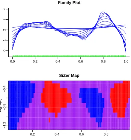
In this paper we are interested in estimating the hazard function, more specifically the hazard for data transformed under a parametric null hypothesis. The idea is to check the adequacy of a postulated model by assessing significance of features in the hazard function of the transformed data. If the model does fit the data then the hazard for the data transformed using the model should be constant, with no monotonic trend neither features. Features such as bumps are characterised by the significant zero crossing of first derivative of the target curve. At a bump there is a zero crossing of the derivative, curve first goes up (positive derivative) and then goes down (negative derivative). Chaudhuri and Marron (1999) described the SiZer analysis from two plots, the “family plot” that is the family of smoothers for the target function indexed by the bandwidth parameter, and a coloured map which displays the scale space inference about the first derivative of the function as follows: for each bandwidth (scale) and value in the support (localization), a confidence interval for the first derivative is calculated and the results about the sign are displayed in a two-dimensional space (map) using a colour code. Consideringnhscales andngridlocalizations, each pixel in thengrid×nhmap is colour-coded as blue if zero is greater than the upper confidence limit (significantly increasing), red if zero is less than the lower confidence limit (significantly decreasing), purple if zero is within the confidence limits (not significantly increasing or decreasing), and gray indicating regions where the data are too sparse to make statements about significance (the effective sample size defined below is less than 5). From the map the features in data are characterized by changes in colour so a change from blue to red displays a significant bump.
Figure1 shows the SiZer analysis for simulated data from a parametric hazard model. The details about how this SiZer has been constructed are given in the next section, now we consider this just as an example to facilitate the understanding of readers not familiarised with this graphical tool. The family plot shows the local linear hazard estimates with different choices of the bandwidth parameter. This gives an idea of the shape of the underlying hazard that the considered smoothing method is able to capture. The bigger bandwidths produce oversmoothed curves showing the general trend in the curve while small bandwidths provide a very detailed description of the hazard with many wiggles. The answer about which features are really there and whether any of these wiggles actually correspond to a significant feature is answered by looking at the colour map in Figure1. This map shows the result of the inference about the first derivative of the hazard. In the vertical axis different smoothing levels in logarithmic scale are represented so drawing a horizontal line at a given value in the range we can see the inference results a that particular value. Following the spirit of the scale space inference real features in data will appear at some of these scales so the analyst should look at all of them to conclude about the significance. On the other hand the horizontal axis shows the values where the hazard (in this case the first derivative) is evaluated, so placing a vertical line in the map we can see the results for the inference at the corresponding point. With this in mind and the colour code described above we can see that the underlying hard is significantly increasing at the beginning (blue colour up to about 0.1), then there is a zero crossing (confidence intervals contain zero between 0.1 and 0.3) and the hazard goes down (red colour up to about 0.5). The change of colours indicates a significant bump around 0.2. Now, if we continue moving the localization up to the right then we can see that a second bump seems to occurs around the value 0.8. Note that the blue colour before 0.8 shows significant increasing interrupted by a zero crossing of the derivative (purple) and ending with significant decrease (red). The data used to construct these plots have been simulated from a distribution with hazard rate obtained as a mixture of Beta functions, that isα(t) =B(t; 6, 2) +B(t; 2, 6), whereB(t;a,b)is the density function of a Beta distribution with
0.0 0.2 0.4 0.6 0.8 1.0
0
1
2
3
4
Family Plot
0.2 0.4 0.6 0.8
−1.2
−0.8
−0.4
log10(h)
SiZer Map
Figure 1.Illustration of SiZer with simulated data.
3.2. SiZer specifications
We now describe the main elements to construct SiZer for inference about a hazard function in the context of aggregated mortality data described in the previous sections. The first choice to define the SiZer analysis is about the family of smoothers to be considered. Our proposal is the local linear estimator of the hazard given in (7), which works from common aggregated mortality data. For the scale space inference about the first derivative we again propose the local linear estimator given in (8), and the estimate of its variance given in (9). With this estimator and its variance we can compute confidence intervals for the first derivative using the expression
b
α0h(t) +q1−p/2 q
d
Var(αb0h(t)),αb0h(t) +qp/2 q
d Var(αb0h(t))
. (10)
Herepis the significance level, andq1−p/2,qp/2are appropriate quantiles. To calculate the quantiles q1−p/2,qp/2 we suggest to use the a Normal approximation. Note that kernel estimates are local averages so the pointwise asymptotic normality of these estimators can be used to construct pointwise confidence intervals, just by taking q1−p/2 and qp/2 equal to the (1−p/2) and p/2 quantiles of the standard Normal distribution, respectively. However SiZer Map is a simultaneous display of statistical inferences, so there is a multiple comparison issue which needs to be addressed. We consider simultaneous inference for SiZer by definingmindependent confidence interval problems, where mreflects the number of independent blocks. Thus, the simultaneous Normal quantiles in SiZer are calculated as follows
q1−p/2=−qp/2=Φ−1
1+ (1−p)1/m 2
! .
reflects the “number of data points in each kernel window”. For the kernel estimators of the intensity theESScan be computed as
ESS(t,h) = ∑ n
i=1Kh(t−Ti)Oi Kh(0)
.
And the number of independent blocks for eachhis estimated as
m= n
avgteDhESS(t,h)
whereavgteDh denotes the average value on the setDh={t:ESS(t,h)≥5}. 3.3. A motivating example to illustrate the strength of SiZer
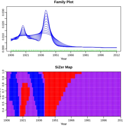
We now show with an example the versatility of SiZer when analysing mortality data. We consider the young male population from Finland and we are interested in evaluating how mortality rate corresponding to this section of the population has evolved along the years. Specifically we estimate mortality rate for male population aged 25 years old from calendar year 1906 to the year 2012. The results are shown in Figure2. According to the plots we can deduce that the mortality rate exhibits a long-term decreasing trend. However two significant features are highlighted in the SiZer map. The colour change blue-purple-red in the first calendar years reveals the existence of a bump around the year 1918. Also another even more prominent bump is located around the years 1943-1945 (see again the colour change blue-purple-red around these years). These two bumps indicate an unusual increase of the mortality rate for the section of population considered here (male population 25 years old) compared to the decreasing evolutionary trend of the mortality along the whole period of time considered (calendar years 1906 to 2012). Notice that this local behavior of the mortality can be explained as a consequence of the two World Wars that took place during the periods 1914–1918 and 1939–1945, respectively.
Year
1906 1921 1936 1951 1966 1981 1996 2012
0.000
0.010
0.020
0.030
Family Plot
Year
log10(h)
1906 1921 1936 1951 1966 1981 1996 2012
0.4
0.5
0.6
0.7
0.8
0.9
1.0
SiZer Map
4. Graphical inspection of a candidate mortality model based on SiZer analysis
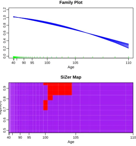
In this section we illustrate the use of SiZer analysis to check the adequacy of a candidate mortality model. We consider an application to real data based on the previous work of Spreeuwet al. (2013) and Gamizet al.(2013). As these authors we analyse mortality data of four countries differing significantly in terms of population size, namely United States (US), United Kingdom (UK), Denmark and Iceland. For each country, the data set consists of female period mortality data, obtained from the Human Mortality Database, and concerning the calendar years 2006 and 2013, the last year from which we have complete datasets for the four countries available at Human Mortality Database. Spreeuwet al. (2013) used these data to check whether the SAINT model that is being used by the major Danish Pension Fund ATP for purposes of asset-liability management is a valid for representing old age mortality. Including the most recent available year 2013 we aim to check whether their conclusions from data in 2006 are still valid in 2013. In the analysis, only the ages from 40 to 110 are included and, as recommended in Spreeuwet al. (2013), we consider a Gamma frailty model as the candidate model to represent the data in the four countries. A visual inspection of a local linear estimator of the density based on transformed data for a single bandwidth choice they showed that the model represented fine the mortality patterns of adult at old ages. With the SiZer analysis introduced in this paper we are now able to assess the significance of these conclusions, avoiding the problem of the non-trivial bandwidth choice, see Gamizet al.(2013) for a discussion of this issue.
The first step to check the adequacy of the model is to estimate the parameters by maximum likelihood. Using the methods described in Section1.2we have derived these estimates for the data in 2006 and 2013, the results are shown in Table1. Then, from the estimated parametric hazardα
b
θ and the corresponding cumulative hazardΛbθ(t) =Rt
Table 1. Maximum likelihood estimations of the parameters of the Gamma frailty hazard model for each country and calendar year. The results concerning the year 2006 have been obtained from Spreeuwet al.(2013).
Country (year) a0 a1 a2 σ
US (2006) -8.1373 0.020140 0.0005402 0.1193
US (2013) -7.5325 0.000114 0.0006905 0.3041
UK (2006) -8.5070 0.01479 0.0006729 0.1632
UK (2013) -8.1421 9.57e-10 0.0007879 0.3704
Denmark (2006) -9.7088 0.06034 0.0003021 0.04007 Denmark (2013) -10.6422 0.07661 0.0002253 0.02559 Iceland (2006) -10.1136 0.05708 0.0003689 0.005556 Iceland (2013) -10.4062 0.05928 0.0003919 0.187948
Age
40 90 95 100 105 110
0.5
0.7
0.9
1.1
Family Plot
Age
log10(h)
40 80 90 95 100 105 110
−0.6
−0.2
0.0
0.2
0.4
SiZer Map
Age
40 90 95 100 105 110
0.6
1.0
1.4
1.8
Family Plot
Age
log10(h)
40 90 95 100 105 110
−0.4
0.0
0.4
SiZer Map
Figure 4.SiZer analysis from mortality data in UK in 2006, transformed under a Gamma frailty hazard model.
Age
40 90 95 100 105 110
0.8
1.2
1.6
2.0
Family Plot
Age
log10(h)
40 90 95 100 105 110
0.5
0.6
0.7
0.8
0.9
SiZer Map
Age
40 90 95 100 105 110
0.8
1.0
1.2
1.4
1.6
Family Plot
Age
log10(h)
40 90 95 100 105 110
0.5
0.6
0.7
0.8
0.9
SiZer Map
Figure 6. SiZer analysis from mortality data in Iceland in 2006, transformed under a Gamma frailty hazard model.
Age
40 90 95 100 105 110
0.5
0.7
0.9
1.1
Family Plot
Age
log10(h)
40 90 95 100 105 110
−0.4
−0.2
0.0
0.2
0.4
SiZer Map
Age
40 90 95 100 105 110
0.6
0.7
0.8
0.9
1.0
1.1
1.2
Family Plot
Age
log10(h)
40 90 95 100 105 110
−0.4
0.0
0.2
0.4
0.6
SiZer Map
Figure 8.SiZer analysis from mortality data in UK in 2013, transformed under a Gamma frailty hazard model.
Age
40 90 95 100 105 110
0.0
0.2
0.4
0.6
0.8
1.0
1.2
Family Plot
Age
log10(h)
40 90 95 100 105 110
0.5
0.6
0.7
0.8
0.9
SiZer Map
0 2 4 6 8 10 12 14
0.0
0.2
0.4
0.6
0.8
1.0
1.2
Age
Family Plot
2 4 6 8 10 12
0.5
0.6
0.7
0.8
0.9
Age
log10(h)
SiZer Map
Figure 10.SiZer analysis from mortality data in Iceland in 2013, transformed under a Gamma frailty hazard model.
5. Conclusions
In this paper we have developed the graphical exploratory tool SiZer map for inference of mortality rates with aggregated data. Using local linear smoothers for the hazard rate and its first derivative the developed SiZer tool is able to detect and confirm the underlying features in the hazard rate such as monotone patterns or local bumps. Besides parametric mortality models can be checked using a transformation approach and afterwards performing the SiZer analysis of the transformed data. The strength of the proposed SiZer analysis has been demonstrated on real mortality data and relevant conclusions have been drawn about a commonly used SAINT frailty model for this kind of data.
Acknowledgments:M.D. Martínez-Miranda acknowledges the support from the Spanish Ministry of Economy and Competitiveness, through grant number MTM2013-41383P, which includes support from the European Regional Development Fund (ERDF). R. Raya-Miranda acknowledges the support from the Spanish Ministry through grant ECO2013-48413-R of the Spanish Ministry of Economy and Competitiveness (co-financed by FEDER).
Conflicts of Interest:The authors declare no conflict of interest.
References
1. Andersen, P., Borgan, O., Gill, R., Keiding, N. (1993).Statistical Models Based on Counting Processes. Springer, New York.
2. Bagkavos, D. (2011). Local linear hazard rate estimation and bandwidth selection. Ann. Inst. Stat. Math. 63, 1019–1046.
3. Chaudhuri, P. and Marron, J.S. (1999). SiZer for exploration of structure in curves. J. Amer. Statist. Assoc., 94, 807–823.
4. Diggle, P. (1985). A kernel method for smoothing point process data,Appl. Statist.,34, 138–147.
6. Gámiz, M.L., Martínez-Miranda, M.D. and Nielsen, J.P. (2013) Smoothing survival densities in practice.
Comput. Statist. Data Anal.,58, 368–382.
7. González-Manteiga, W., Martínez-Miranda, M.D., Raya-Miranda, R. (2008). SiZer Map for inference with additive models. Stat. Comput.18, 297–312.
8. Jarner, S.F. and Kryger E.M. (2011) Modelling adult mortality in small populations: The SAINT model.ASTIN Bulletin41(02) 377-418
9. Marron, J. S. and Zhang, J.T. (2005). SiZer for smoothing splines.Computat. Statist.,20, 481–502.
10. Nielsen, J. P. and Tanggaard, C. (2001). Boundary and bias correction in kernel hazard estimation.Scand. J. Statist.,28, 675–698.
11. Nielsen, J. P., Tanggaard, C., and Jones, M.C. (2009). Local linear density estimation for filtered survival data.Statistics,43, 167–186.
12. Park, C. and Kang, K.-H. (2008). SiZer analysis for the comparison of regression curves. Comput. Statist. Data Anal.,52, 3954–3970.
13. Park, C., Hannig, J., and Kang, K. (2009). Improved SiZer for Time Series.Statist. Sinica,19, 1511–1530. 14. Park, C., Hannig, J., and Kang, K.-H. (2014). Nonparametric Comparison of Multiple Regression Curves in
Scale-Space.J. Comput. Graph. Statist.,23, 657-677.
15. Park, C., Hernandez-Campos, F., Le, L., Marron, J. S., Park, J., Pipiras, V., Smith, F. D., Smith, R. L., Trovero, M. and Zhu, Z. (2011). Long Range Dependence Analysis of Internet Traffic.J. Appl. Stat.,38, 1407–1433. 16. Park, C., Lee, T. C. M. and Hannig, J. (2010). Multiscale exploratory analysis of regression quantiles using
quantile SiZer.J. Comput. Graph. Statist.,19, 497–513.
17. Park, C., Marron, J. S. and Rondonotti, V. (2004). Dependent SiZer: goodness of fit tests for time series models. J. Appl. Stat.,31, 999–1017
18. R Core Team (2015). R: A language and environment for statistical computing. R Foundation for Statistical Computing, Vienna, Austria. URLhttps://www.R-project.org/.
19. Rondonotti, V., Marron, J. S., and Park, C. (2007). SiZer for time series: a new approach to the analysis of trends.Electronic J. Statist.,1, 268–289.
20. Spreeuw, J., Nielsen, J.P. and Jarner, S.J. (2013) A visual test of mixed hazard models.SORT,37, 149–170 21. Wang, J. L., Muller, H.G. and Capra, W. B. (1998). Analysis of oldest-old mortality: Lifetables revisited.
Ann. Statist.28, 126—163.
c