Leverage and Volatility Feedback E¤ects and Conditional
Dependence Index: A Nonparametric Study
Yiguo Sun and Ximing Wuy
April 5, 2018
This paper studies the contemporaneous relationship between S&P 500 index returns and log-increments of the market volatility index (VIX) via a nonparametric copula method. Speci…cally, we propose a conditional dependence index to investigate how the dependence between the two series varies across di¤erent segments of the market return distribution. We …nd that: (a) the two series exhibit strong, negative, extreme tail dependence; (b) the negative dependence is stronger in extreme bearish markets than in extreme bullish markets; (c) the dependence gradually weakens as the market return moves toward the center of its distribution, or in quiet markets. The unique dependence structure supports the VIX as a barometer of markets’mood in general. Moreover, applying the proposed method to the S&P 500 returns and the implied variance (VIX2), we …nd that the nonparametric leverage e¤ect is much stronger than the
nonparametric volatility feedback e¤ect, although, in general, both e¤ects are weaker than the dependence relation between the market returns and the log-increments of the VIX.
Keywords: Conditional Dependence Index; Kendall’s Tau; Leverage E¤ect; Nonparametric Copula; Tail Dependence Index; Volatility Feedback E¤ect.
JEL Classi…cation: C13; C22; G1
1
Introduction
Investors witnessed severe downturn in the U.S. stock market in the second half of year 2008 when the mood of the bearish market was often cited through an implied volatility index–the VIX, a trade mark held by the Chicago Board Options Exchange (CBOE). The VIX is designed to retrieve market’s estimate of average S&P 500 index volatility over the subsequent 22 trading days. As bearish markets frequently observed counter-movements between S&P 500 index prices and the VIX, the VIX earned itself a reputation of market barometer of investors’fear (see Figure 1).1Motivated by this observation, we join the traditional …nance literature to study the leverage and volatility feedback e¤ects via nonparametric method, where asymmetric GARCH-in-mean type of models are popularly used in such study (see Bekaert and Wu (2000), and references therein).
Corresponding author; Department of Economics and Finance, University of Guelph, ON N1G2W1, Canada; E-mail address: [email protected].
yDepartment of Agricultural Economics, Texas A&M University, College Station, TX 77843, U.S.A.; E-mail
address: [email protected].
1“Fears Takes a Holiday: VIX at 7-Month Low”. The Wall Street Journal, December 4, 2010.
To explain a stylized fact of stock markets–the asymmetric volatility: Volatility responds more to a drop in the value of a stock (index) than an increase of equal amount in the value of the stock (index), two popular hypotheses have been put forward such as the leverage and volatility feedback e¤ects hypotheses; see Black (1976), Bollerslev and Zhou (2006), Campbell and Hentschel (1992), Christie (1982), French, Schwert and Stambaugh (1987), Schwert (1989), among many others. From empirical …nancial econometrics point of view, the two hypotheses explain opposite causality between stock price movements and volatility. So, which direction of causality is stronger? The answer is inconclusive; see, Bekaert and Wu (2000) , Bollerslev et al. (2006), Figlewski and Wang (2001), among others. Moreover, there is no agreement on which data set shall be used. For example, the literature has seen volatility measured by historical volatility, conditional volatility, realized volatility and implied volatility. Noticeable research study has been made to learn the information content of the four di¤erent volatility measures; for example, Anderson and Bollerslev (1998), Christensen and Prabhala (1998), Fleming (1998), Blair et al. (2001), Poon and Granger (2003), Becker, Clements, and McClelland (2009), Jiang and Tian (2005), among many others.
In this paper, we use the VIX as the measure of volatility. The VIX is published by the CBOE almost continuously each trading day such that it is public information available to all investors. Therefore, it will be a public interest to learn more about how the two publicly observable series, the S&P 500 index and its implied volatility index (or VIX), interact with each other. Also, in empirical …nance literature, the relationships between VIX (or the VIX changes) and market returns are popularly studied in semiparametric or parametric regression framework, which can su¤er potential model misspeci…cation problem. For example, Bollersleve and Zhou (2006) and Bekirosa, Jlassic, Naouid, and Uddine (2017) estimate the leverage and volatility feedback e¤ects from several competitive parametric models and notice that the magnitude of these e¤ects is very sensitive to the underlying model used for the analysis. In this paper, we therefore introduce a model-free approach to reinvestigate the causality between the implied variance (or the changes in VIX) and the market returns, by estimating the joint density functions of the two variables of interest. Speci…cally, we apply the nonparametric copula technique developed by Wu (2010) to estimate the joint density functions.
pay particular attention to the leverage e¤ect of the market returns on the market expected future volatility. Here, the concept of theleverage e¤ ect is extended to the impact of the (contemporaneous and lagged) S&P 500 index returns on the implied variances.
One advantage of our research is that we attach the leverage e¤ect with the performance of S&P 500 index, while traditional research, using asymmetric GARCH-type models to study the leverage e¤ect, tends to de…ne the leverage e¤ect with respect to a predetermined reference point, usually zero.2 Interestingly, we …nd that the leverage e¤ects exhibit a W shape across di¤erent segments of S&P 500 index return distribution (see the red curve in Figure 5). To our knowledge, this is an interesting new …nding that has not been documented in the …nance literature: When studying the leverage e¤ects of market returns, one needs to look beyond how market volatility reacts to positive or negative market returns.
The volatility feedback e¤ect documented states that market returns are positively correlated with market volatility, and the returns are high (low) if the anticipated volatility increases (de-creases). GARCH-in-mean type of models are usually used to test the volatility feedback e¤ect (e.g. Porterba and Summers (1986), French, Schwert, and Stambaugh (1987), Campbell and Hentschel (1992), Glosten, Jagannathan and Runkle (1993)), where the coe¢ cient for volatility e¤ect is as-sumed to be a positive constant. Bekaert and Wu (2000) did allow market volatility to bear a varying risk premium when modeling excess stock (index) returns of Japanese market by assum-ing a conditional version of the CAPM based on the riskless debt model; however, the volatility feedback e¤ect is di¢ cult to be estimated accurately as stated in their paper. In this paper, the conditional dependence index proposed in Section 4 is a model-free measure of the volatility feed-back e¤ect. We …nd that the volatility feedfeed-back e¤ect (the green line in Figure 5) is a U-shape curve as the squared VIX moves across di¤erent segment of its distribution. In contrast to Bakaert and Wu’s (2000) …nding, but consistent with Engle and Ng (1993) and references in Bollerslev, Litvinova, and Tauchen (2006), we …nd that the volatility feedback e¤ect is generally smaller than the leverage e¤ect (see Figure 5).
Most researchers agree that the implied variance,VIX2, has a long-memory of its past, while S&P 500 market returns have a very short memory of its past; see the sample autocorrelations of the implied variances and of the market returns reported in Table 1 over the period of 01/01/1990 and 12/29/2017. We therefore decompose the logarithm of the implied variance into two components: its previous day value and its daily increment (named rvix in this paper). The results in Table 3 show that the log-increment of the VIX has very short memory comparable with the market return. Since the relation between market returns and the implied variance is a balanced or net outcome of the relation of the market returns with each component of the implied variance, we then explore the instantaneous relation between the short-memory component of the implied variance and the market returns.3 That is, we investigate not only the leverage and volatility feedback
2As an exception, Wu and Xiao (2002) studied the asymmetry of the volatility response curve via a generalized
partially linear regression model of the VIX on S&P 100 index, which is a semiparametric approach.
3
e¤ects along the line of the traditional …nance literature, but also study the relation between the log-increments of the VIX and the market returns. Our empirical …ndings are consistent with our intuition: we observe considerable contemporaneous dependence between S&P 500 index returns and the logarithm changes of the VIX (see the black curve in Figure 5), which is bigger than both the leverage and volatility feedback e¤ects in terms of magnitude in general.
The strong daily, negative, asymmetric relation between the market returns and the increments of the market volatility is also found in Gibot (2005) and Hibbert et al. (2009) in a simple linear regression model framework and Bekirosa, Jlassic, Naouid, and Uddine (2017) in a linear quantile regression setup. Our analysis provides several additional noteworthy results: (a) the two series exhibit strong, negative, extreme tail dependency; (b) the negative dependency is stronger in extreme downturn markets than in extreme bullish markets; (c) the dependency gradually weakens as the market return moves toward the center of its distribution, or in quiet markets. These results imply that the simple linear regression model with a dummy variable to account for positive or negative market returns may not be su¢ cient to capture the extreme tail relation between the log-increments of the VIX and the S&P 500 index returns and that the average relation implied by the linear regression model may understate the relation of the two series in extreme market conditions.
The rest of the paper is organized as follows. Section 2 presents the data and summary statistics. Section 3 discusses the nonparametric estimation of copula joint densities and presents the tail dependence indexes of interest. In Section 4, we propose a conditional dependence index to study the leverage and volatility feedback e¤ects and the relation between market returns and the log-increments of the VIX. To check on the robustness of the results, we conduct subsample analysis by splitting the data into four subsample periods. We conclude in Section 5. All tables and …gures are delayed to the end of the paper.
2
Data and Descriptive Statistics
We downloaded daily S&P 500 index prices from DataStream and daily implied volatility (or VIX) from the CBOE. The data span from January 2, 1990 (the …rst date that the VIX is available) to December 29, 2017. The VIX is designed to provide a benchmark market volatility index measuring the market’s aggregate view of the average market volatility over the subsequent 22 trading days, calculated from both at-the-money and out-of-the-money S&P 500 option contracts satisfying some volume conditions (Whaley, 1993, 2000) via a model-free method developed by Demeter…, Derman, Kamal and Zou (1999) and originated from the seminal work of Breeden and Litzenberger (1978). Detailed information about the VIX can be found at http://www.cboe.com.
The VIX is frequently cited as a barometer of investors’ fear, and this view of the implied volatility has found strong popularity among the investor community. A high VIX beyond 40 is usually linked to a severe bear market while a low VIX value to a market with more con…dence. The …rst time that the VIX surpassed the value of 40 was on August 31, 1998, a year marked by Russia’s currency devaluation and national debt moratorium and the collapse of the Long Term Capital Management in the U.S.A. The number of transaction days with the VIX value exceeding 40 is 15, 4, 10, 63, 61, 3, 11, and 1 in the year of 1998, 2001, 2002, 2008, 2009, 2010, 2011, and 2015, respectively. On November 20, 2008, the VIX reached its record high of 80.86, marking an unprecedented …nancial crisis faced by global …nancial markets.
We plot the two data series in Figure 1. For the data period under consideration, the two indexes moved in opposite directions in 77.68 percent of the total transaction days. Splitting the data according to the directions of the S&P 500 index price movements, we observe this: of 77.08 percent of the total 3,285 transaction days that the S&P 500 index fell, the VIX gained; of 78.30 percent of the total 3,765 transaction days that the S&P 500 index gained, the VIX fell. We also see a signi…cant increase in counter-movements between the two indexes during extremely bearish market periods; for example, the two series move in opposite directions 84.92%, 88.93%, and 80.15% of the transaction days in the year of 1998, 2008, and 2009, respectively.
LetPtand V IXt2 be the S&P 500 index price and the implied variance at datet, respectively.4
We construct the daily S&P 500 index return and the log-increment of the VIX as follows:
rspt= 100 ln (Pt=Pt 1) and rvixt= 100 ln (V IXt=V IXt 1): (1)
Table 3 reports the summary statistics of the implied variance, S&P 500 index returns, and log-changes of the VIX. It is noted that rvixt has a slightly lower average but signi…cantly higher
variation than rspt during the sample period. We then split the data according to the sign ofrspt
and calculate the upside and downside averages and sample standard deviations for bothrspt and
rvixt. Interestingly, we observe that both series exhibit stronger volatility in the downturn markets
than in the upturn markets. In the downturn markets, the market index performed considerably worse than in the upturn markets, and the opposite holds true for the VIX index. Also, the implied variance,V IXt2, is on average lower and less volatile when the S&P 500 index prices went up than when the S&P 500 index prices came down.5
Next, we use three dependence measures betweenrspandrvixto examine the counter-movements between the S&P 500 index prices and the VIX values, including Pearson’s correlation coe¢ cient,
4The VIX is the implied standard deviation of near future average market index volatility. Therefore, the implied
variance equals the squared value of the VIX. 5
Kendall’s tau,6 and = Pr (rspt rvixt<0). Kendall’s tau reveals a strong negative (or positive)
association between the two series if it is close to negative (or positive) one, and a weak association if it is close to zero. Kendall’s tau equals zero, if the two series are independent, but it may not hold true vice versa. As for 2 [0;1], the probability that the two series move in opposite directions, the closer is to one, the stronger is the negative association between rspt and rvixt. We report
our estimates in the fourth to sixth columns in Table 4. The sample correlation betweenrvixt and
rspt ranges from -0.878 in 2015 to -0.450 in 1995 and Kendall’s tau ranges from -0.727 in 2015 to
-0.295 in 1995. The negative dependence was more prominent in the past eighteen years of the 21th century than in the 1990s. For the entire sample period under consideration, there are 77.7 percent of chances that the S&P 500 index prices and the VIX values moved in opposite directions, and this number peaked at 88.9 percent in 2008 and bottomed at 63.9 percent in 1995. Roughly speaking, the worse the market is, the stronger is the negative dependence.
The second and third columns of Table 4 report the sample correlation and Kendall’s tau of (V IX2
t; rspt), which give an overall measure of the relation between the expected near future
market aggregate risk and current market aggregate return. All these statistics are negative and signi…cantly di¤erent from zero at the 5% level, but less prominent than those between rvixt and
rspt. The overall lower negative relation between rspt and V IXt2 is not a surprise, given the fact
that the V IXt2 is a long-memory process while the rspt has a very short serial correlation with
itself; see Table 3.
To sum up, Table 4 indicates a signi…cant negative relation between the market returns and the log-increments of the VIX (and market implied variance). At the same time we also notice that the negative relation is stronger when the market index performs poorly than when the market index performs well. It implies that an overall negative association between the two series cannot tell the full story of how the two series relate. This observation motivates us to examine the joint distribution of the two series in the next section.
3
Copula Function and Tail-Dependence Index
To further our understanding of the dependence relationship between the S&P 500 returns and the log-increments of the VIX and between the S&P 500 returns and theV IX2, we use the device of copula to decompose their joint probability density functions (or p.d.f.’s). According to the Skalar’s
6Kendall’s tau is given by
= Pr[(X1 X2)(Y1 Y2)>0] Pr[(X1 X2)(Y1 Y2)<0]
= 2 Pr[(X1 X2)(Y1 Y2)>0] 1,
where(X1; Y1)and(X2; Y2)are continuous random vectors drawn from the same joint cumulative distributionF(x; y);
theorem, the joint density of two continuous random variablesX andY can be written as
f(x; y) =fX(x)fY (y)c(FX(x); FY (y)), (2)
where X has a marginal p.d.f. fX(x) and a cumulative distribution function (or c.d.f., hereafter)
FX(x), andY has a marginal p.d.f. fY (y)and a c.d.f. FY (y). As a function of the c.d.f.’s ofX and
Y, the copula density function, c(FX(x); FY (y)), captures completely the dependence structure
between X and Y. We refer interested reads to Nelsen (1999) for a thorough treatment of the copula method and Cherubini, Luciano, and Vecchiato (2004) for applications in …nance.
As a powerful tool to measure extreme co-movement across di¤erent international stock markets and di¤erent assets, copulas have been widely used in empirical …nance literature to explore non-linear tail dependence; e.g., Chollete et al. (2011), Liu, Ji, and Fan (2017) and references therein. However, it is common practice for researchers assume a certain parametric copula function in their analysis, which can create model misspeci…cation problem. The commonly used parametric copula families (e.g., Gaussian copula, Student’s t copula, and Fréchet copula) implicitly impose speci…c dependence structure betweenXandY, which may not be supported by empirical data. For exam-ple, Gaussian copula density assumes that the two variables have a constant correlation regardless of whether X and Y are around the median or tails of their respective distributions. This depen-dence structure imposed by Gaussian copula evidently is not consistent with the fact documented in the preceding section that the dependence between the S&P 500 index returns and the implied variance is stronger during severe bearish market periods, which is featured with unusually high implied variance and low S&P 500 index returns, than during quite market periods with relatively low implied variance. Therefore, in this paper, to avoid misspecifying the dependence structure of
rspt; V IXt2 and of(rspt; rvixt), we shall adopt a nonparametric copula method proposed by Wu
(2010) to estimate their copula density functions. Allowing the data to speak out their true rela-tion, Wu (2010) proposes an exponential series copula density estimator (henceforth, ESE) without preassuming parametric form of dependence structure between two series of interest.
Below, we brie‡y explain the ESE estimator, denoting u =FX(x) and v =FY (y) to simplify
our notation. Firstly, to guarantee a positive copula density function, we approximate it by
c(u; v; ) = exp
0
@ X
0<i+j m
ijuivj+ 0 1
A,0 u; v 1, (3)
where m is a positive integer, and 0 = lnR01R01exp P0<i+j m ijuivj dudv is a constant to
ensure that c(u; v; ) integrates to unity. The ESE can be viewed as a series approximation of the log density, and the functional form of c(u; v; ) is determined by m, which is the order of polynomials of the log copula density.
Secondly, to estimate the parameters, = ( 0;f i;j : 1 i+j mg), in (3), we apply Jaynes’
entropy
max
Z 1
0 Z 1
0
c(u; v; ) logc(u; v; )dudv (4)
subject to the following integration-to-unity condition and mmoment conditions Z 1
0 Z 1
0
c(u; v; )dudv= 1 (5)
Z 1
0 Z 1
0
uivjc(u; v; )dudv=E uivj , 0< i+j m. (6)
Finally, in practice, letting the number of moments increase with sample size at an appropriate rate and replacing the population moments in (6) with their corresponding sample moments, one obtains a consistent nonparametric estimator of the underlying copula density function. The sample moments are su¢ cient statistics of the underlying distribution, and the MLE estimator of the ME density can be shown to be asymptotically e¢ cient (Crain, 1974).
Jaynes’ (1957) ME Principle suggests that one can use a number of su¢ cient statistics that depict the copula density function. For example, if X and Y are drawn from a bivariate normal distribution, it is well-known that knowing the mean and variance su¢ ce to identify the Gaussian copula density function; i.e.,mwill be two. As one does not know the true copula density function in practice, an incorrectly selected set of su¢ cient statistics would lead to misleading inference on the dependence relation between variables of interest. How does the choice of the set of su¢ cient statistics a¤ect our estimation of the copula density function? The intuition is this: a smaller set of su¢ cient statistics may omit important, relevant information associated with some missing su¢ cient statistics, which will evidently lead to biased inference on the true dependence structure between the two variables of interest; on the other hand, a larger than necessary set of su¢ cient statistics will incorporate redundant information associated with the inclusion of some non-useful extra moments, in‡ating the variation in the estimation of ’s because of the loss of degree of freedoms. Therefore, the set of su¢ cient statistics, or more precisely, the order ofm of polynomial in the exponent of equation (3) shall be selected carefully. In fact, one can view mas a smoothing parameter in the framework of nonparametric density estimation. In this paper,m is selected in a data-driven manner according to the Akaike Information Criterion (AIC), an information criterion balances the trade o¤ between accuracy and complexity in model construction.7
Now, let the marginal cumulative distribution functions of rvixt, V IXt2 and rspt denoted by
urvix;t Frvix(x),uV IX2;t FV IX2(x), and vt Frsp(x), respectively.8 Since these quantities are
7Of course, one can also apply other nonparametric methods to estimatec(u; v). For example, one can use a kernel
estimator or an empirical distribution based estimator. We choose to use the ESE estimator as Wu (2010) suggests
that the ESE estimator su¤ers less bias than the kernel estimator when(u; v)taking values near the boundary of the
space of unit square[0;1]2. In addition, the empirical distribution based estimator may be less smooth than the ESE
estimate.
8
To simplify our notation, we will drop the subscripttfromurvix;t,uV IX2;t, andvtwhen we detact no confusion
usually unknown, we replace them by their frequency estimates, i.e. F^rvix(x) = 1=TPTt=1I(rvixt
x), F^V IX2(x) = 1=TPTt=1I(V IXt2 x), and F^rsp = 1=TPTt=1I(rspt x), respectively. Several
bene…ts could result from the one-to-one transformation of the variable of interest via its cumulative distribution function: a) it can e¤ectively mitigate potential outlier problems in the nonparametric estimation; b) as a measure of the likelihood of the occurrence of an event, probability provides a direct way of capturing market relative status than the raw data value does across time, which is the upmost important in our study of the relationship between the two indexes in a quick-changing market environment. Furthermore, the study of the transformed data (v; urvix) and (v; uV IX2),
instead of the raw data, provides a key tool to consolidate historical study of similar situations so that we can discuss relation between two series according to event probabilities. This point will be illustrated in the next section where we discuss the full sample and subsample results.
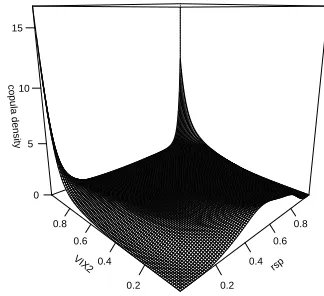
In Figure 2, we plot the estimated copula density functions for (v; urvix) with m = 5 and
for (v; uV IX2) with m = 7, where m’s are selected to minimize the AIC. The preliminary results
in Section 2 indicate strong negative association between rspt and rvixt without identifying the
sources of the observed relation. The left panel in Figure 2 suggests that the negative dependence between the S&P 500 index returns and the log-increments of the VIX is largely driven by the counter-movements at the two tails, since the bulk of the copula density is along the anti-diagonal line and spikes up at the two corners. In other words, the co-movements of the opposite tails of the two marginal distributions contribute signi…cantly to the negative dependence between the S&P 500 index returns and the log-increments of the VIX. In addition, the density at the upper left corner in this graph, corresponding to the case of low market index returns and high VIX changes, is larger than its counterpart associated with high market index returns and low VIX changes. Except for the two tails along the anti-diagonal line in the [0;1]2 unit square, the copula density appears to be rather symmetric.
The right panel in Figure 2 plots the estimated copula density for(v; uV IX2), where we observe
that the S&P 500 index returns and theV IX2 are strongly dependent when the implied variance is extremely high or its c.d.f. is close to one. The dependence is stronger when the market returns are extremely low and the implied variance is very high than when both the market returns and implied variance are extremely high. Or, put in another word, the estimated copula density indicates that the S&P 500 index returns and theV IX2 is highly dependent during high volatile markets and the dependency is stronger in a panic triggered high volatile market than an exhilarated high volatile market. On the other hand, we observed that the dependence between the two variables ‡attens out when the implied variance locates between its 10th percentile to its 80th percentile. We also note that the estimated copula density hump up a bit when the implied variance locates to its left tail.
3.1 Tail Dependence Index Between rsp and rvix
The joint copula density of (rsp; rvix) in Figure 2 clearly exhibits the left-right and right-left tail dependence between the S&P 500 index returns and log-increments of the VIX. To quantify the prominent tail dependence between the two series, one naturally wants to investigate the probability with which rvix lies to the lower or upper tail area when rsp resides in the opposite tail area.9
As the dependence occurs at the tails, such probability is usually called tail dependence index (or TDI, henceforth). This idea is not new and has been studied in di¤erent …elds. For example, Poon, Rockinger, and Tawn (2004) studied one particular tail index using extreme value theory, although they focus on the limit cases; that is, TDI( ) = Pr Y < FY1( )jX < FX1( ) when ! 1 or !0, whereFX1( )andFY 1( )are the(100 )thpercentile ofX andY, respectively. Taking clues from the estimated copula density seen in the left panel of Figure 2, we focus on the following two TDIs that capture the co-movements of opposite tails of(rsp; rvix):
TDI1( ) = Pr rvix < rvix jrsp > rsp1 = Pr (urvix< jv >1 ), (7)
TDI2( ) = Pr (rvix > rvix1 jrsp < rsp ) = Pr (urvix >1 jv < ), (8)
wherervix andrsp are the(100 )thpercentile of the return seriesrvixandrsp, respectively. Taking = :01 and = :05 respectively, we obtain TDI1(:01) = :078, TDI2(:01) = :101,
TDI1(:05) =:285, and TDI2(:05) =:354 from the estimated copula density exhibited in Figure 2.
If the two series were independent, we would obtain TDIj( ) = forj = 1;2. Therefore, the fact
that TDIj( ) is substantially higher than indicates strong negative tail dependence betweenrsp
and rvix series. In particular, our results suggest that extreme movements in the S&P 500 index are associated with extreme movements of the VIX to the opposite direction with high probabilities. In addition, the fact that TDI1( )<TDI2( )for both =:01and =:05reveals that the VIX asymmetrically responds to extreme movement of the S&P 500 index prices. The probability that the VIX increases abruptly when the market index faces free-fall is much higher than the probability that the VIX falls back when the market index price enjoys strong rebound. The asymmetry is consistent with the stylized fact frequently documented in the …nance literature that the market tends to respond more to bad news than to good news of equal magnitude, although this stylized fact is described from our point view of tail dependence indexes.
The fact that the tail dependence is more pronounced when the market is in turmoil explains why the VIX is dubbed as the Investor Fear Gauge.
9
We also calculated the tail dependence index on the conditional probability thatrsp lies to its tail area given
thatrvix resides in the opposite tail area. As this mirrors relation to the one reported in the paper does not bring
3.2 Tail Dependence Index Between rsp and V IX2
As the right panel of Figure 2 exhibits a prominent dependence between the S&P 500 index returns and implied variances when the latter reside at the right tail of its distribution, we introduce the following four TDIs:
g
TDI1( ) = Pr rsp > rsp1 jV IX2> V IX12 = Pr (v >1 juV IX2 >1 ) (9)
g
TDI2( ) = Pr rsp < rsp jV IX2> V IX12 = Pr (v < juV IX2 >1 ) (10)
g
TDI3( ) = Pr V IX2> V IX12 jrsp > rsp1 = Pr (uV IX2 >1 jv >1 ) (11)
g
TDI4( ) = Pr V IX2> V IX12 jrsp < rsp = Pr (uV IX2 >1 jv < ) (12)
where V IX2 is the (100 )th percentile of the V IX2 series. We use = :01 to illustrate the meaning of each index. First, TDIg1(:01) and TDIg2(:01) measure the probabilities that the S&P 500 returns reside to the respective right and left 1% tail of the return distribution in an extremely volatile market condition. Second,TDI3g ( )andTDI4g ( )give the probabilities that the market sees extremely high volatility with the implied variance falling to its upper 1% tail of its distribution in an extremely high and low market return periods.
By construction, TDIg1( )and TDIg2( ) re‡ect thevolatility feedback e¤ ect of market volatility on market returns at extreme situation, while TDIg3( ) and TDIg4( ) re‡ect the leverage e¤ ect of market returns on market volatility at extreme situations. Of course, the leverage and volatility feedback e¤ects referred here are extended from the traditional meaning of the two e¤ects.
Again, we take =:01 and :05. From the estimated copula density function shown in Figure 2, we calculate TDIg1(:01) = 0:089, TDIg2(:01) = 0:137, TDIg1(:05) = 0:198, TDIg2(:05) = 0:307,
g
TDI3(:01) = 0:076,TDIg4(:01) = 0:119, TDIg3(:05) = 0:199, andTDIg4(:05) = 0:308. As TDIgj( )>
for all the cases studied, we see apparent tail dependence between the market returns and market implied variances, although the tail dependence of the implied variances on the market returns is generally weaker than that of the changes of VIX on the market returns. In addition,
g
TDI1( )<TDIg2( )and TDIg3( )<TDIg4( ) for both =:01and =:05, indicating asymmetric tail dependence between the market returns and implied variances; i.e., the TDIs are stronger when the market returns lie to the left tail of than to the right tail of the return distribution.
3.3 Contemporaneous and Lagged Conditional Distributions
The tail dependence index only describes the probability of the occurrence of one rare event given that of another rare event. In this section, we aim to extract more information from the data by estimating the conditional cumulative distribution (or c.c.d.f., henceforth) functions via the non-parametric copula method. Speci…cally, letA be a subset of[0;1]. We are interested in estimating the conditional c.d.f.’s listed in Table 1.
Table 1: The List of Conditional Cumulative Distributions of Interest Case Conditiondal c.d.f. Description
C1 F(urvix;tjvt h2A) the conditional c.d.f. of urvix;t givenvt h2A
C2 F(vtjurvix;t h 2A) the conditional c.d.f. of vt givenuvix;t h2A
C3 F uV IX2;tjvt h2A the conditional c.d.f. of uV IX2;t given vt h 2A
C4 F vtjuV IX2;t h 2A the conditional c.d.f. of vt givenuV IX2;t h 2A
Note: h= 0 and 1;A= [0; :05],[:45; :55], and [:95;1]
A = [0; :05], [:95;1], and [:45; :55], we aim to study the behavior of the conditional c.d.f.’s under extreme and moderate market conditions. If each pair of variables among v, urvix and uV IX2
were drawn from a bivariate normal distribution, one would expect the conditional c.d.f. invariant with respect to the choice of A. Also, the choice of h = 0 or 1 is used to measure the strength of contemporaneous relation relative to lag-one relation. Examining Figures 3 and 4, we aim to visually test two hypotheses summarized in Table 2.
Table 2: The Hypotheses of Interest The null Hypothesis on F(ytjxt h2A) Implication
H10: F(ytjxt h2A) coincides with the 45-degree line yt is independent of xt h when xt h2A
H20: F(ytjxt h2A) does not vary with A (xt h; yt) are jointly normally distributed
Note: (xt; yt h) = (urvix;t; vt h),(vt; urvix;t h), uV IX2;t; vt h , or vt; uV IX2;t h ;
h= 0;1;A= [0;0:05];[:45; :55], and [:95;1]
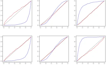
Reading Figure 3, we observe that both the hypotheses H10 and H20 fail to hold for all the contemporaneous c.c.d.f.’s. Evident deviations of the c.c.d.f.’s from the 45-degree line result from strong tail dependence between the log-increments of the VIX and the market returns. On the other hand, the inter-dependence between the two series are rather mild during quite market periods. Evidently, the results in Figure 3 support varying dependence relation between the two series across di¤erent market conditions, which suggests the inadequacy of …tting the data with bivariate normal distribution with a constant correlation. Whenh= 1, the hypothesis H10 holds roughly true for all the lag-one conditional c.d.f.’s (or l.c.c.d.f.’s, hereafter), as they are all close to the 45-edgree line. Combining our observations, we see strong daily contemporaneous dependence between the market returns and log-increments of the VIX and very weak if nothing at all one-day lag dependence. Actually, when we push h up to 20, we did not see signi…cant lag dependences between the two series.
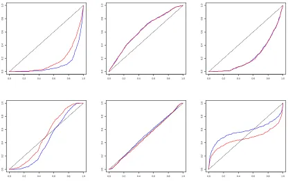
Let us next look at Figure 4. Di¤erent from Figure 3, the c.c.d.f.’s and l.c.c.d.f.’s are very close to each other, which is especially true for the conditional c.d.f.’s ofuV IX2;t given vt h2A (in the
l.c.c.d.f.’s of vt given uV IX2;t h 2 [:45; :55]. Overall, the c.c.d.f.’s and l.c.c.d.f.’s of uV IX2;t given
vt h2A deviate from the 45-degree line more than those of vt givenuV IX2;t h 2A.
To sum up, we observe strong contemporaneous left-right and right-left tail dependence between
rspand rvix, signi…cant contemporaneous and lagged tail dependence of the VIX2 on the market returns, and mild tail dependence of the market returns on the VIX2. Although useful, these qualitative assessments are largely based on smoothing and visualization of data. In the next section, we propose a conditional dependence index to formally quantify the conditional dependence between each pair of series of interest among the market returns, the log-increments of the VIX, and the VIX2.
4
Conditional Dependence Index
As we discuss above, Figures 3 and 4 plot several estimated conditional distribution functions of u
given v 2A, where A is a nonempty subinterval of the interval [0;1]. If u and v are independent of each other when v 2 A, we have F(ujv 2 A) = F(u) for all u 2 [0;1] so that knowing the information fv 2 Ag does not help us make better predictions about u. On the other hand, the further is the conditional c.d.f. away from the 45-degree line, the higher is the dependency between
u and v 2 A. Therefore, it is natural to use the area between the conditional c.d.f. and the 45-degree line as a proxy of the predictive power of v 2 A on u. In doing so, we are able to learn under what circumstances u and v are most dependent as v moves across its distribution function. Consequently, we can make inference on the relation between the pair of variables of interest conditional across di¤erent market status.
Hence, we propose a conditional dependence index (or CDI, henceforth) which equals twice of the area between a conditional c.d.f. and the 45-degree line, given the fact of v 2 A. Thus, the index is de…ned as a functional ofA:
G(A) = 2
Z 1
0 j
F(ujv2A) ujdu= 2E[jF(ujv2A) uj]. (13)
Evidently, for any given sub-interval A [0;1], 0 G(A) 1, where G(A) = 0 means indepen-dence between u and v given v2A, and the dependence of u on v2Agrows as G(A) gets closer to the unity. Partitioning the [0;1] interval into twenty equal-width intervals, we calculate G(A)
for each interval and report the results in Table 5 for bothh= 0 and h= 1.
Now, we illustrate the estimation method and the test for G(A) = 0 for the case thatG(A) =
2E[jF(urvix;tjvt h2A) urvix;tj], the CDI of the log-increments of the VIX on the market returns.
(And the method is also applied to the other cases.) We denote the estimator ofG(A) by G^(A), which is given by
^
G(A) = 2
n
n
X
t=h+1
^
F(utjvt h2A) ut , (14)
=Pr (vt h 2A) by its empirical conditional distribution, ^
F(utjvt h2A) =
n 1Pnt=1I(urvix;t ut; vt h2A)
n 1Pn
t=1I(vt h2A)
=
n 1Pnt=1I rvixt Frvix;t1 (ut); rspt h2Frspt1 h(A)
n 1Pn
t=1I rspt h2Frspt1 h(A)
, (15)
with the total sample size, n=7,055,I( )being the indicator function, andFrvix;t( )andFrspt h( )
being the unconditional c.d.f.’s ofrvixt and rspt h, respectively. ^
G(A) is a consistent estimator of G(A) as supu2[0;1] F(ujv 2A) F^(ujv2A) = op(1) and
the sample mean is a consistent estimator of a population mean, given the fact that both series are stationary. Actually,G^(A) =G(A) +Op n 1=2 .
Next, we are interested in testing the null hypothesis of G(A) = 0 against the alternative hypothesis ofG(A)>0. If the null hypothesis holds true, we can show thatpn F^(ujv2A) u
converges to a normal random variable with zero mean and …nite variance. Under the alternative hypothesis, we expectpn F^(ujv2A) u =Op(pn). Therefore, we expect pnG^(A) = Op(1)
under the null hypothesis and pnG^(A) =Op(pn) under the alternative hypothesis. However, to
conduct the test, we need to obtain proper critical values. As the distribution ofG^(A) under the null hypothesis does not have a simple formula, we propose to use bootstrap critical values.
Bootstrap critical values. Should the alternative hypothesis hold true, the realization of
the log-increment of the VIX is a¤ected by the realization of the market return. Therefore, the temporal ordering of the market return matters in the calculation of G^(A). However, should the null hypothesis hold true, we have F^(ujv2A) = n 1Pnt=1I rvixt Frvix;t1 (u) , the empirical
c.d.f. of rvixt, which does not depend on the realization of the market returns, nor does G^(A).
Therefore, the temporal ordering of the market returns should not matter in the calculation ofG^(A), should the null hypothesis hold true. Basing on these observations, we propose to obtain bootstrap samples by randomly shu- e the market returns while keeping the order of the log-increments of the VIX. As a result, the bootstrap sample contains the raw data on rvix and the randomly shu- ed market return data, rsp , and the bootstrap sample size is the same as the original sample size, n=7,055. To obtain the bootstrap critical value at the signi…cance level of 5% for example, we repeat 500 bootstrap procedures and use the 95th percentile of the 500 bootstrap statistics,G^ (A), to approximate the critical value, whereG^ (A) is the bootstrap estimate ofG(A) using (15).
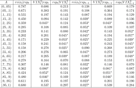
In Table 5, we report G^(A) for six cases: the CDIs ofrvixt given rspt h,V IXt2 given rspt h,
rspt given V IXt h2 for h = 0 (capturing contemporaneous dependence) and for h = 1(capturing
one day lagged dependence).10 We divide the interval [0;1] into twenty intervals with equal in-crement of .05. In Table 5, we marked the insigni…cant CDI estimates at the 5% level with an
1 0We calculated but decided not to report the CDIs of rsp
t given rvixt has the extra results do not add more
asterisk. The …fth column of Table 5 indicates little dependence of the log-increments of the VIX on previous day’s market index performance. Combining the second and …fth columns, we see close contemporaneous but less noticeable lagged relation between the changes of the VIX and the market returns. In contrast, the relation between implied variance and market returns are rather persistent but become weaker in general over time, where the persistent relation may result from the long-memory properties of the implied variance.
To enhance the readability of the results given in Table 5, we plot the contemporaneous CDIs in Figure 5. The black line shows how the distribution of the log-increments of the VIX depends on the market return as the market return moves from its lower 5% tail, (.05,.10], (.10,.15,],..., to its upper 5% tail, where each probability interval contains equally 5% of the data. It shows a general U-shape curve, bottoming at the interval of (.45,.50]–around the median of the market returns. The dependence of the distribution of the log-increments of the VIX on the market returns grows as market returns go farther away from its median, although the dependences grow faster with steeper slope when the market return falls below its median value than when the market return grows above its median value ( for the full sample, the daily market average return is 0.04584%). At the extreme market cases, the CDI of the log-increments of the VIX takes the highest value .787 when the market return falls below its lower 5% tail, which is higher than .680 when the market return grows beyond its upper 5% tail. The …nding re‡ects market’s asymmetric attitude toward an extreme down market and an extreme upper market: investors in general feel more nervous in the former than the latter situation.
Below, we will link our empirical results found in this section to the traditional …ndings on the leverage and volatility feedback e¤ects. Here, we refer to the leverage e¤ ect as the dependence of the implied variance on the market returns at lag one and the volatility feedback e¤ ect as the dependence of the market returns on the implied variance at lag one.
The leverage e¤ect. The red line in Figure 5 shows how the distribution of the V IXt2
the latter can be relatively accurately estimated during quite market periods, where the implied variance equals the sum of variance premium and the conditional variance of market returns as de…ned in Bekaert and Hoerova (2014) who found that the variance premium is a component of the implied variance to predict future market returns.
The volatility feedback e¤ect. The green line in Figure 5 shows how the distribution of
rspt depends on V IXt2 1, where we see a much ‡atter convex curve than the black curve. The right most column of Table 5 shows that the volatility feedback e¤ects are insigni…cant at the 5% signi…cance level when the market return falls into the probability interval of [.3,.35) to [.6,.65). It means that we would not …nd noticeable volatility feedback e¤ect if we …t the data with a mean regression model. This result may be used to explain why empirical works cannot …nd volatility feedback e¤ects with GARCH-in-mean model; e.g., Campbell and Hentschel (1992).
Comparing the three curves, we …nd noticeably higher dependence between the market returns and log-increments of the VIX than the leverage and volatility feedback e¤ects, except for a higher leverage e¤ect when the market return is moving around its medium value. This result encourages the econometric modeling of the market returns and log-changes of the VIX besides the leverage and volatility feedback e¤ects. In addition, the volatility feedback e¤ect is weaker than the leverage e¤ect with some exceptions. This result may support the …ndings in Christie (1982) and Bekaert and Wu (2000) that neither the leverage e¤ect nor the volatility feedback e¤ect can be the sole explanation of the volatility asymmetry observed from stock markets.
To sum up, we …nd strong dependence between rvix and rspand the dependence is stronger in volatile market periods than in relatively quiet market periods. As the VIX reveals market’s expectation on the future 30-day volatility, our results indicate that investors make sharp revision on their belief of market risks during extreme volatile market periods, and that the revision is less noticeable during tranquil market periods. It again con…rms that the negative association between the S&P 500 index prices and the VIX mainly come from tail events.
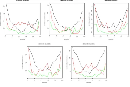
To check on how robust our …ndings are, we also conduct subsample analysis, where we split the sample period into …ve subperiods: January 2, 1990 to December 31, 1994; January 1, 1995 to December 31, 1999; January 1, 2000 to December 31, 2004; January 1, 2005 to December 31, 2009; January 1, 2010 to December 31, 2017.11 Figure 6 plots the estimated CDIs for the four subsample periods. In general, the subsample results are similar to the full sample results shown in Figure 5, except for the …rst subperiod.
5
Conclusions
nonparametric leverage e¤ect exhibits a W-shape curve as the implied variance moves from the left to the right tail of its distribution. Second, nonparametric volatility feedback exhibits a U-shape curve as the S&P 500 index returns moves across the return distribution. Third, the nonparamet-ric leverage e¤ect in general is higher than the nonparametnonparamet-ric volatility feedback e¤ect, except in relatively quite market conditions.
The VIX index squared, as a risk-neutral measure of market volatility, is market’s best estimate of average future realized volatility over ensuing 22 trading days plus avolatility risk premium, as documented by Todorov (2009), Bollerslev and Zhou (2005), among many others for other implied volatility indexes than S&P 500 implied volatility. Bakshi and Madan (2006) provide a theoretical model to explain that the VIX squared (or the implied variance) depends on historical skewness and kurtosis of return distributions and market risk aversions. Therefore, the log-increments of the VIX may re‡ect market’s revision on risk aversion and average future realized volatility as the S&P 500 index price changes. The empirical results in this paper indicate that the contemporaneous dependence between market’s revision on risk aversion and average future realized volatility and the market returns are stronger than the leverage and the volatility feedback e¤ects when the market’s movement deviates from its medium range.
Applying Wu’s (2010) ESE nonparametric copula estimator in Section 3, we …nd strong tail dependency among the market returns, log-increments of the VIX and the VIX2. From Figures 3 and 4, we get an impression that the dependence relations among each pair of the three series vary with market conditions and are strongest during extreme bearish markets.
References
[1] Aboura, S., N. Wagner (2016). Extreme asymmetric volatility: Stress and aggregateasset prices.Journal of International Financial Markets, Institutions & Money 41, 47-59.
[2] Bakshi, G. and D. Madan (2006). A theory of volatility spreads. Management Science 52, 1945-1956.
[3] Bekaert, G. and G. Wu (2000). Asymmetric volatility and risk in equity markets.The Review of Financial Studies 13, 1-42.
[4] Bekaert, G. and M. Hoerova (2014). The VIX, the variance premium and stock market volatil-ity. Journal of Econometrics 183, 181–192.
[5] Becker, R., A.E. Clements, and A. McClelland (2009). The jump component of S&P 500 volatility and the VIX index.Journal of Banking & Finance 33, 1033-1038.
[7] Black, F. (1976). Studies of stock market volatility changes. Proceedings of the American Statistical Association, Business and Economics Statistics Section, 177-181.
[8] Blair, B.J., S.H. Poon, and S.J. Taylor (2001). Forecasting S&P 100 volatility: the incremen-tal information content of implied volatilities and high-frequency index returns. Journal of Econometrics 105, 5-26.
[9] Bollerslev, T., Litvinova, J., and G. Tauchen (2006). Leverage and volatility feedback e¤ects in high-frequency data.Journal of Financial Econometrics 4, 353-384.
[10] Bollerslev, T. and H. Zhou (2006). Volatility puzzles: a simple framework for gauging return-volatility regressions.Journal of Econometrics 131, 123-150.
[11] Breeden, D.T., and R.H. Litzenherger (1978). Prices of state contingent claims implicit in option prices. Journal of Business 51, 621-651.
[12] Campbell, J.Y. and L. Hentschel (1992). No news is good news: an asymmetric model of changing volatility in stock returns.Journal of Financial Economics 31, 281-318.
[13] Cherubino, U., E. Luciano, and W. Vecchiato (2004). Copula Methods in Finance. John Wiley & Sons, Ltd.
[14] Chollete, L., V. de la Peña, C. Lu (2011). International diversi…cation: A copula approach.
Journal of Banking & Finance 35, 403-417.
[15] Christie, A.A. (1982). The stochastic behavior of common stock variances-value, leverage and interest rate e¤ects.Journal of Financial Economics 10, 407-432.
[16] Christensen, B.J. and N.R. Prabhala (1998). The relation between implied and realized volatil-ity.Journal of Financial Economics 50, 125-150.
[17] Crain, B. R. (1974). Estimation of distributions using orthogonal expansions. Annals of Sta-tistics 16, 454-463.
[18] Demeter…, K., E. Derman, M. Kanial, and J. Zou (1999). More than you ever wanted to know about volatility swaps.Quantitative Strategies Research Notes, Goldman Sachs.
[19] Engle, R.F., and V.K. Ng (1993). Measuring and testing the impact of news on volatility.
Journal of Finance 48, 1749–1778.
[20] Fleming, J. (1998). The quality of market volatility forecasts implied by S&P 100 index option prices.Journal of Empirical Finance 5, 317-345.
[22] Giot, P. (2005). Relationships between implied volatility indexes and stock index returns.The Journal of Portfolio Management 31,92-100.
[23] Glosten, L.R., R. Jagannathan, and D.E. Runkle (1993). On the relation between the expected value and the volatility of the nominal excess return on stocks.Journal of Finance 48, 1779-1801.
[24] Hibbert, A.M., R.T. Daigler, and B. Dupoyet (2008). A behavioral explanation for the negative asymmetric return-volatility relation.Journal of Banking & Finance 32, 2254-2266.
[25] Liu, B., Q. Ji, Y. Fan (2017). A new time-varying optimal copula model identifying the de-pendence across markets.Quantitative Finance 17, 437-453
[26] Jaynes, E.T. (1957). Information theory and statistical mechanics.Physics Review 106, 620-30.
[27] Jiang, G.J. and Y.S. Tian (2005). The model-free implied volatility and its information content.
The Review of Financial Studies 18, 1305-1341.
[28] Nelsen, R.B. (1999). An Introduction to Copulas. Springer-Verla, New York, Inc.
[29] Poon, S. and C. Granger (2003). Forecasting volatility in …nancial markets: a review. Journal of Economic Literature 41, 478-539.
[30] Poon, S., M. Rockinger, and J. Tawn (2004). Extreme value dependence in …nancial markets: diagnostics, models and …nancial implications.The Review of Financial Studies 17, 581-610.
[31] Poterba, J.M., and L.H. Summers (1986). The persistence of volatility and stock market ‡uc-tuations.American Economic Review 76, 1142–1151.
[32] Todorov, V., 2009. Variance risk-premium dynamics: the role of jumps. TheReview of Finan-cial Studies 23, 345-383.
[33] Whaley, Robert E. (1993). Derivatives on Market Volatility: Hedging Tools Long Overdue.
Journal of Derivatives 1, 71-84.
[34] Whaley, Robert E. (2000). The Investor Fear Gauge. Journal of Portfolio Management 26, 12-17.
[35] Wu, G. and Z. Xiao (2002). A generalized partially linear model of asymmetric volatility. Journal of Empirical Finance 287-319.
Appendix:
Tables and Figures
Table 3: Summary Statistics (01/02/1990-12/29/2017)
Variable x x x+ ^ ^ ^+
V IX2 450.178 492.787 412.208 479.277 538.629 415.808
rvix 0.018 3.410 -3.010 5.888 5.432 4.454
rsp 0.019 -0.791 0.742 1.137 0.882 0.802
(1) (2) (3) (4) (5) (6)
V IX2 .971 .947 .933 .916 .908 .896
rvix -.091 -.081 -.033 -.034 -.014 -.030
rsp -.049 -.069 .024 -.025 -.035 .005
a. x=average return,x =downside average return over times whenrsp <0,
x+=upside average return over times when rsp 0;
b. ^=sample standard deviation, ^ =downside sample standard deviation over times whenrsp <0, ^+=upside sample standard deviation over times whenrsp 0.
c. ^(h) is the sample autocorrelation of lag hand the 5% critical value equals 0.023. Also, the Ljung-Box statistics with six lags areQrsp(6) = 45:58; Qrvix(6) = 110:72, and QV IX2(6)
Table 5: Conditional Dependence Indexes
A rvixtjrspt V IXt2jrspt rsptjV IXt2 rvixtjrspt 1 V IXt2jrspt 1 rsptjV IXt2 1
(0; :05) 0.787 0.686 0.213 0.138 0.669 0.179
[:05; :1) 0.671 0.383 0.191 0.108 0.364 0.174
[:1; :15) 0.555 0.197 0.143 0.087 0.194 0.129
[:15; :2) 0.450 0.094 0.142 0.039 0.089 0.136
[:2; :25) 0.359 0.045 0.124 0.053 0.043 0.096
[:25; :3) 0.285 0.108 0.085 0.052 0.109 0.107
[:3; :35) 0.233 0.141 0.080 0.042 0.143 0.052
[:35; :4) 0.202 0.201 0.045 0.045 0.194 0.057
[:4; :45) 0.171 0.229 0.053 0.025 0.225 0.039
[:45; :5) 0.158 0.241 0.041 0.025 0.243 0.045
[:5; :55) 0.158 0.278 0.025 0.090 0.268 0.018
[:55; :6) 0.206 0.276 0.065 0.047 0.273 0.033
[:6; :65) 0.217 0.205 0.039 0.087 0.189 0.048
[:65; :7) 0.278 0.164 0.070 0.088 0.153 0.071
[:7; :75) 0.307 0.146 0.081 0.032 0.146 0.070
[:75; :8) 0.362 0.080 0.101 0.046 0.081 0.087
[:8; :85) 0.424 0.052 0.124 0.025 0.051 0.109
[:85; :9) 0.480 0.046 0.169 0.028 0.046 0.146
[:9; :95) 0.611 0.195 0.197 0.022 0.201 0.190
[:95;1) 0.680 0.537 0.297 0.027 0.539 0.284
Figure 1: Raw Data Plot (01/02/1990-12/29/2017; black: S&P 500 Index; red: VIX)
1990 1995 2000 2005 2010 2015
500
1000
1500
2000
2500
Time
S&P 500
VIX
6
17
29
40
51
63
74
Figure 2: Joint Copula Density Functions Estimated by Nonparametric Copula Method (Left: rvixt and rspt; Right: V IXt2 andrspt)
rsp
0.2 0.4
0.6 0.8
rvix
0.2 0.4 0.6 0.8
copula density
2 4 6 8
rsp
0.2 0.4
0.6 0.8
VIX2
0.2 0.4 0.6 0.8
copula density
Figure 3: Conditional Ccumulative Distribution Function Estimates (blue: h= 0; red: h= 1) (Upper row: rvixjrsp; Lower row: rspjrvix. Left: A=(0,.05]; Middle: A=[.45,.55]; Right: A=[.95,1))
0.0 0.2 0.4 0.6 0.8 1.0
0.0
0.2
0.4
0.6
0.8
1.0
0.0 0.2 0.4 0.6 0.8 1.0
0.0
0.2
0.4
0.6
0.8
1.0
0.0 0.2 0.4 0.6 0.8 1.0
0.0
0.2
0.4
0.6
0.8
1.0
0.0 0.2 0.4 0.6 0.8 1.0
0.0
0.2
0.4
0.6
0.8
1.0
0.0 0.2 0.4 0.6 0.8 1.0
0.0
0.2
0.4
0.6
0.8
1.0
0.0 0.2 0.4 0.6 0.8 1.0
0.0
0.2
0.4
0.6
0.8
Figure 4: Conditional Ccumulative Distribution Function Estimates (blue: h= 0; red: h= 1) (Upper row: VIX2 jrsp; Lower row: rspjVIX2;Left: A=(0,.05]; Middle: A=[.45,.55]; Right: A=[.95,1))
0.0 0.2 0.4 0.6 0.8 1.0
0.0
0.2
0.4
0.6
0.8
1.0
0.0 0.2 0.4 0.6 0.8 1.0
0.0
0.2
0.4
0.6
0.8
1.0
0.0 0.2 0.4 0.6 0.8 1.0
0.0
0.2
0.4
0.6
0.8
1.0
0.0 0.2 0.4 0.6 0.8 1.0
0.0
0.2
0.4
0.6
0.8
1.0
0.0 0.2 0.4 0.6 0.8 1.0
0.0
0.2
0.4
0.6
0.8
1.0
0.0 0.2 0.4 0.6 0.8 1.0
0.0
0.2
0.4
0.6
0.8
1.0
Figure 5: Full Sample Conditional Dependence Index Estimates (black: rvixjrsp; red: VIX2jrsp; green: rspjVIX2)
0.0 0.2 0.4 0.6 0.8 1.0
0.0
0.2
0.4
0.6
0.8
probability
conditional dependence inde
Figure 6: Subsample Conditional Dependence Index Estimates (black: rvixjrsp; red: VIX2jrsp; green: rspjVIX2)
0.0 0.2 0.4 0.6 0.8 1.0
0.2
0.4
0.6
0.8
01/01/1990−12/31/1994
probability
conditional dependence inde
x
0.0 0.2 0.4 0.6 0.8 1.0
0.2
0.4
0.6
0.8
01/01/1995−12/31/1999
probability
conditional dependence inde
x
0.0 0.2 0.4 0.6 0.8 1.0
0.1
0.2
0.3
0.4
0.5
0.6
0.7
01/01/2000−12/31/2004
probability
conditional dependence inde
x
0.0 0.2 0.4 0.6 0.8 1.0
0.2
0.4
0.6
01/01/2005−12/31/2010
probability
conditional dependence inde
x
0.0 0.2 0.4 0.6 0.8 1.0
0.2
0.4
0.6
0.8
01/01/2010−12/31/2016
probability
conditional dependence inde