Wave Dissipation in Mangroves
Parameterization of the drag coefficient based on field data.
M.Sc Thesis Graduation Committee:
J.M. Hendriks dr. ir. C.M. Dohmen-Janssen
February 2014 ir. E.M. Horstman
University of Twente dr. D.S. van Maren
2
ACKNOWLEDGEMENTS
This report is the result of my M.Sc. thesis performed at Twente University and Deltares, as the final part of the master, Water Engineering and Management at Twente University.
The data used in this thesis have been collected and provided by Erik Horstman, who also closely collaborated in this thesis. I would like to thank him for his contribution and all the time he has put into providing me with feedback.
Large part of the execution of this M.Sc. thesis has been performed at Deltares research institute in Delft. They kindly provided me with the workspace and knowledge needed in order to bring this thesis to a good result. I would like to thank everyone at Deltares who helped me with parts of this thesis, but especially Claire Jeuken for making all necessary arrangements, and Bas van Maren for providing valuable contacts and feedback when needed.
Next, I would like to thank Tomohiro Suzuki, for the insight he provided in the SWAN vegetation module he created, the suggestions he made for interesting relations to investigate, and the time and effort he has put into the meetings and feedback.
In general I would like to thank for the time and effort they have put into helping me to come to this final result, all the members of my graduation committee:
dr. ir. C.M. Dohmen-Janssen ir. E.M. Horstman
dr. D.S. van Maren dr. ir. T. Suzuki
Last but not least I would like to thank my friends and family for supporting me throughout my study, and providing me with feedback when needed.
Jurjen Hendriks
5 In which CD is the drag coefficient (-), and KCM is the KC number with Mazda length scale (-) as
defined before.
When implementing this equation in the SWAN model, small improvements were obtained compared to the old situation with a single constant drag coefficient for each transect. This new equation slightly increased the R-squared and correlation values of predicted vs. observed energy dissipation rates. However, the greatest improvement lies in the fact that both transects available in the data are represented by the same equation, rather than both having a different value in the old situation. This is a first step towards more generic modelling of vegetation-induced wave dissipation.
7
7.2 Comparison to literature ... 68
7.3 Vertical variation of vegetation... 68
7.4 Data limitations ... 69
7.5 Sensor accuracy and precision ... 69
7.6 Unaccounted parameters ... 69
7.7 Unaccounted physical processes ... 69
7.8 Representing formulation ... 70
8 Conclusions ... 72
9 Recommendations ... 74
Literature ... 76
Appendix I: Overview of Field studies ... 80
Appendix II: Overview of the main characteristics of the acquired data (Narra, 2012) ... 84
Appendix III: Analysis of sensor abnormality ... 86
Appendix IV ... 90
9
FIGURE 1 DISTRIBUTION OF MANGROVES WORLDWIDE (ADAPTED FROM GIRI ET AL. 2011)
Mangrove vegetation consists of trees and shrubs that are able to survive in saline
environments. A great distinction between mangroves and normal trees comes from the aerial roots found at mangroves (Tomlinson 1986). Since mangroves are situated at intertidal flats which are submerged periodically, the mangroves need these aerial roots for oxygen uptake. The most common root types found in mangroves are pneumatophores, knee roots and stilt roots (figure 2). The aerial roots of mangroves will be submerged by the sea at least part of the tidal cycle .
FIGURE 2 MANGROVE ROOT SYSTEMS (FROM LEFT TO RIGHT): PNEUMATOPHORES, KNEE ROOTS AND STILT ROOTS (DE VOS 2004)
1.1.2 MANGROVE WAVE INTERACTION
Waves propagating through vegetation fields lose part of their energy due to the interaction with the vegetation (Mendez and Losada, 2004). As waves propagate through mangroves, they will experience resistance from the trunks, aerial roots and in some cases the canopy as well. Due to the often extensive root systems of mangroves, this drag can become quite significant and wave attenuation in mangroves has been found to contribute to the protection of the shore (Danielson et al., 2005). Burger (2005) investigated this interaction, and the most important variables playing a role in this attenuation process. He concluded that the actual wave dissipation depends on both vegetation characteristics and hydraulic conditions.
10
FIGURE 3 WAVE ENERGY SPECTRUM, SHOWING THE RELATIVE ENERGY OF DIFFERENT WAVE TYPES COMPARED TO EACH OTHER (REEVE ET AL., 2004)
1.1.3 PHYSICAL PROCESSES
11
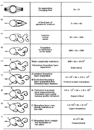
FIGURE 4 FLOW AROUND A CYLINDER AT DIFFERENT FLOW REGIMES (SUMER AND FREDSOE, 2006)
Although the energy loss is temporally and spatially varying, in general a time averaged value is used in literature. Since the timescale in which the variations in flow speed (and thus energy loss) take place is small (cf. the wave period), for the total average energy loss over time this will have no effects.
1.1.4 FIELD STUDIES
Over the last decades, several field studies have been performed into the attenuation of waves in mangroves (e.g. Brinkman et al 1997, Mazda et al 1997a, Massel et al, 1999, Mazda et al 2006, Quartel et al 2007, Vo-Luong and Massel 2006,2008, and Bao 2011). Even though each of these field studies measured and represented wave attenuation in a different way, during all of these studies the wave attenuation effects of mangroves have been proven. The rates of wave
14
FIGURE 5 SWAN MODEL OVER VO-LUONG AND MASSEL (2006) DATA (SUZUKI ET AL, 2011B)
1.1.7 DRAG COEFFICIENT
The vegetation’s drag coefficient is often used as a calibration parameter to obtain model results that compare favourably with field observations. However, research has shown that this drag coefficient is not constant, but can vary depending on different variables. From general flow theory around cylinders, the Reynolds number can be found to influence the drag coefficient (e.g. Dennis and Chang 1970, Son and Hanratty 1968). When looking more specifically at drag experienced by vegetation under wave conditions, an adaptation in the Reynolds number has been proposed by Mazda et al (1997b), including vegetation characteristics in the Reynolds number, which they showed to have more correlation with the drag coefficient. Another
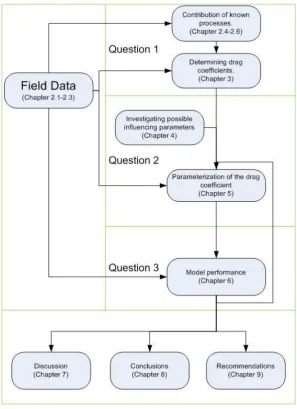
17 Chapter two will present the data used in this study, including an analysis of the wave
attenuation observed in this data. The chapter will start with a general introduction of the available data, with information about the data itself and the locations and manner in which the data was acquired. Next, general trends in the data will be investigated to see whether these are in line with the expectations. Also, subsets of the data will be analysed to check for consistency and possible unknown effects or errors in the data. Furthermore this chapter will answer question 1.1, by seeing to what extend bottom friction on itself can represent the energy losses witnessed.
After the exploration of the data, chapter three describes the process of determining the drag coefficients from this data. Furthermore, this chapter will provide an overview of the drag coefficients derived from the data.
In chapter four, literature will be used in order to construct a list of variables that might possibly influence the drag coefficient. This list is used in chapter five in order to find a parameterization for the drag coefficient. In chapter six, this parameterization will then be validated.
The report will end with a discussion, conclusions, and recommendations for further investigations into the subject.
18
2 DATA EXPLORATION
To fulfil the aims of this thesis, field data is needed, including both vegetation characteristics and wave data. Field data acquired by Horstman et al. (2012) and pre-processed by Narra (2012), are used. This chapter will look both at the acquiring of this data as well as the quality of the data itself and the processes observed in the basic data.
First, this chapter summarizes how the data was collected. Secondly, the data itself will be introduced and visualized. Thirdly, the quality of the available data will be investigated. Next, an estimation will be made to see how much of the energy dissipation can be attributed to wave-mangrove interaction. Finally, spectral differences in wave attenuation will be discussed.
2.1 DATA DESCRIPTION
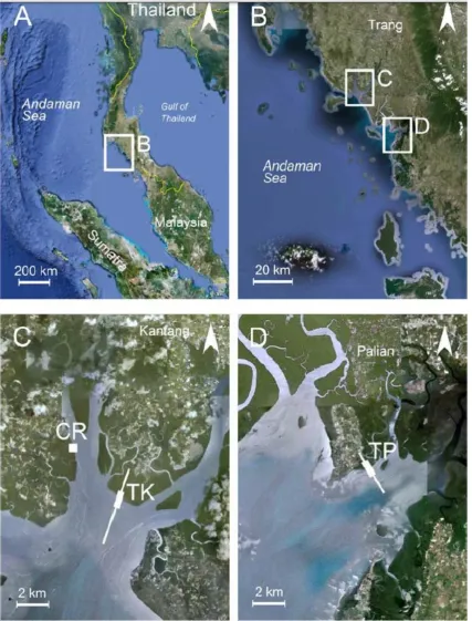
The data used for this thesis is a set of field data on wave attenuation in mangroves, which has been acquired by Horstman et al. (2012)/Horstman (2014) at two study sites, situated at the coast of Trang province in Thailand. These locations have been selected by Horstman (2014) because of the pristine condition of the mangroves in this region, a high vegetation diversity and a characteristic gradient in forest vegetation.
Two wave transects were selected, based on vegetation characteristics, positioning, and practical reasons. Both transects have multiple zones of vegetation, with either Avicennia or Rhizophora as the dominant species. Examples of these species can be found in figure 7. The locations and positioning of these transects are presented in figure 8. Although both transects show undisturbed mangroves, there are significant differences between the sites as well. The first transect, located in the Kantang district, is exposed to open sea, while the second transect, located in the Palian district, is situated at the side of a river estuary. Furthermore, there is a difference in the slopes between the two transects. And last, there is a difference in mangrove densities.
19
22
2.2 DATA INTRODUCTION
The field data acquired by Horstman et al.(2012) have been used by Narra (2012) to analyse the relations between mangrove density and wave dissipation. Narra found a positive correlation between vegetation density and energy dissipation over 100 metre distance. Furthermore, he found a negative correlation between water depth and energy dissipation. However, he also shows this relation differs per zone, and the variation in the data makes the uncertainty of the conclusions quite significant. All in all though, when comparing with previous studies, Narra concludes that the data shows similar trends.
Narra showed a clear decrease of energy for both transects when considering the average data (figure 11). However, one exception can be seen in sensor 4 for the Palian transect.
FIGURE 11 WAVE ENERGY OVER THE TRANSECTS (NARRA 2012) CENTRAL LINES SHOWING THE AVARAGE VALUES WHILE THE UPPER EN LOWER LINE REPRESENT THE STANDARD DEVIATION
From the raw data it is clear the measurements have been taken place in a wide range of
conditions. For example the significant wave heights observed at the first sensor range from 1 to 43 centimetres for the Palian transect and 1 to 32 centimetres for the Kantang transect. The experienced peak periods seen for the transects do also vary. Peak periods range from 1.5 to around 18 seconds for both transects. An overview of the main statistics of the data as determined by Narra (2012) can be found in appendix II.
23
FIGURE 12 WAVE ENERGY SPECTRA AT THE PALIAN TRANSECT (MEASUREMENT 1)
FIGURE 13 WAVE ENERGY SPECTRA AT THE KANTANG TRANSECT (MEASUREMENT 1)
24 waves are visible at around 0.12 Hz, which is equivalent to a period of about 8.3 seconds.
Furthermore, at the Palian transect an energy peak can be seen at very short waves (0.65 Hz). These differences in wave energy density spectra are most likely caused by the positioning of the transects.
2.3 DATA QUALITY
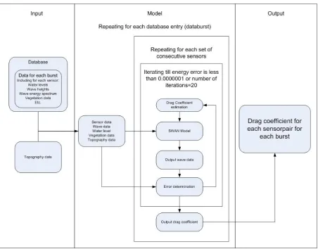
To get an initial idea of the quality of the data (and especially the variation within the data), bottom friction factors have been determined with Matlab, which represents the observed energy dissipation between two consecutive sensors. The determination of these friction factors is based on the bottom friction approach as introduced before, with an iterative process in which the friction factor is calibrated based on the energy calculated for the next sensor, compared to the measured energy at this sensor. An example of the results of such a run is plotted in figure 14.
FIGURE 14 FRICTION FACTOR VS SIGNIFICANT WAVE HEIGHT FROM FIELD DATA
These plots show that the variation in friction factors is large and some sensors might be erroneous, resulting in negative friction factors. The variation can be explained easily by accuracy of the sensors used to measure the wave conditions. The accuracy of these sensors is only about 1 cm, thus at wave heights of 5 centimetres, there can be an error of 20% in the measured wave heights. For small energy losses between two sensors, these losses can easily turn into energy gains with this error. Even though lots of the scatter in this plot can be
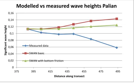
27 the sensor data, while the modelled datasets cannot predict this. These effects must therefore be caused by the presence of the mangroves.
2.5 SPECTRAL DIFFERENCES IN WAVE ATTENUATION
In the previous analysis only the significant wave height and the corresponding frequency have been used. However, wave dissipation might vary over wave frequencies. To check whether this is the case, the percentage of energy loss between consecutive sensors has been calculated for each frequency band and plotted (see figure 21).
As expected, in general the energy losses between sensors 4-5 and 5-6 (high density mangroves) are higher than for the other two. Another clear trend which can be observed, is that more dissipation takes place at the higher frequencies (shorter waves). For these short waves, the influence of mangroves seems to become negligible, most of these waves are damped over the mudflat before even reaching the mangroves. The influence of the mangroves itself is most visible at the frequencies below 0.5 Hz. For the longest waves, dissipation seems to decrease rapidly, showing almost no energy losses in dense mangroves for waves at 0.05 Hz, and energy gains at this frequency for the mudflat and low density mangroves.
From this figure the preliminary conclusion would be that the influence of mangroves varies over the frequency bands. However, since only the total energy loss is considered, which also includes contributions of other processes (e.g. bottom friction), the spectral differences can in theory as well be caused by these other processes.
28
2.6 CONCLUSIONS
32
FIGURE 18 SCHEMATIZATION OF THE CALIBRATION PROCESS
3.3 RESULTS
In order to get a usable set of drag coefficients the extremes have to be filtered out. Any drag coefficient value which is at the set limits should be removed from the dataset. Considering the calibration procedure, CD values below (or about 10-4 ), or CD values above
are not possible. Any C
D values outputted at this values are therefore
considered to end up outside the set limits. For the Kantang transects there are 270 drag coefficient values which are in the low limit of the simulation and 0 in the high limit of the simulation. For the Palian transect this were 602 in the low limit and 2 in the high limit. These values are removed from the data leaving a total of 11363 entries.
The average drag coefficients between sensors at the different transects, are in line with the values found in literature, with average CD values between 2 and 4 (see table 6 and 7). The
standard deviations though, are considerably high. When comparing the Kantang and Palian transects, the average CD values follow the same trend, while the standard deviations at the
33
TABLE 6 AVERAGE DRAG COEFFICIENTS AND STANDARD DEVIATIONS FOR THE FIELD DATA AT THE PALIAN TRANSECT
Palian Average CD Standard deviation
Sensor 2-3 4.0 4.1
Sensor 3-4 4.0 4.1
Sensor 4-5 0.84 0.52
Sensor 5-6 0.59 0.34
TABLE 7 AVERAGE DRAG COEFFICIENTS AND STANDARD DEVIATIONS FOR THE FIELD DATA AT THE KANTANG TRANSECT
Kantang Average CD Standard deviation
Sensor 2-3 2.4 2.4
Sensor 3-4 4.2 2.6
Sensor 4-5 3.2 1.6
Sensor 5-6 1.6 1.3
For both transects a decrease in CD is observed with increasing densities, indicating some effects
35
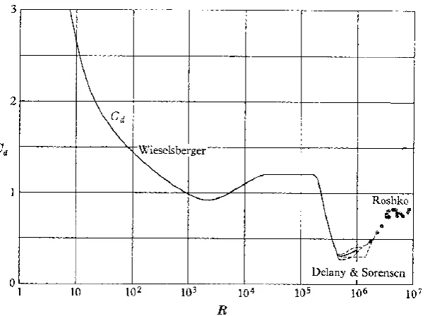
FIGURE 19 DRAG COEFFICIENT VS. REYNOLDS NUMBER, A COLLECTION OF DATA FROM DIFFERENT STUDIES (ADAPTED FROM ROSHKO, 1960)
Mazda et al. (1997b), investigated the relation between the drag coefficient and the Reynolds number for vegetation in general, again showing a clear relation between Reynolds number and drag coefficient. However, in the data from Mazda et al., the drag coefficient seems to be limited to a value of around 15, at low Reynolds numbers, rather than infinity (see figure 20). This might indicate an exponential function rather than a power function, but due to the limited range of this data set (with lowest Reynolds values being around 102) this cannot be verified.
These differences in the type of relations between the drag coefficient and the Reynolds number at low Reynolds numbers, show that there currently is no single definition for the drag
36
FIGURE 20 DRAG COEFFICIENT VS. REYNOLDS NUMBER (MAZDA ET AL., 1997B)
4.1.1 IMPLEMENTATION
The Reynolds number, as seen before, can be defined by the following equation:
In general, for oscillatory flow, the characteristic length scale (LC) in this equation is generally
defined as the maximum horizontal movement of a particle under the influence of the wave. This is defined as:
This characteristic length scale includes no vegetation data. For this reason Mazda et al (1997b), came up with a different definition for this characteristic linear dimension:
In this equation Vc is the control volume (m3), Vm is the vegetation volume within this control
volume (m3), and Ap is the projected surface area of this vegetation (m2), perpendicular to the
37 Reynolds number, thus this might give better results. However, since no other uses of this linear dimension have been found in literature, both definitions will be assessed in this thesis.
4.2 KC-NUMBER
Mendez and Losada (2004), demonstrated the importance of the Keulegan-Carpenter number, especially for the drag coefficient in case of vegetation. The Keulegan-Carpenter number has been introduced by Keulegan and Carpenter (1958), to account for the effects of changing values of drag coefficients with changing flow velocity or size of cylinders in oscillating fluids. The Keulegan-Carpenter number is defined as:
In which u is the maximum flow velocity (m/s), T is the period of the oscillation (s) and Lc is the
characteristic length scale (m). For cylinders this length scale is generally defined as the diameter.
Mendez and Losada (2004), calculated a bulk drag coefficient and KC values for a total of 115 data points, and obtained a clear relation. They specified the following relation:
This relation had a 76% correlation according to their calculation.
As can be seen in the plot they made (figure 21), some of their variation was caused by different values of (the vegetation height relative to the water depth). In order to include this effect they suggested an adaptation to the Keulegan-Carpenter number (Q):
With this adaptation for the KC number the following relation with the drag coefficient was found:
38
FIGURE 21 DRAG COEFFICIENT VS KEULEGAN CARPENTER NUMBER (MENDEZ AND LOSADA, 2004)
4.2.1 IMPLEMENTATION
As seen before, (Mendez and Losada, 2004) have shown the correlation between the KC number and the drag coefficient.
The period of the oscillation used for calculating the KC number, is the period corresponding to the maximum flow velocity. For this reason the peak period is implemented as the period of the oscillation.
In order to determine the influence of the KC number it is important to decide what vegetation characteristics will be used to compute the KC number. The KC number can differ between different vegetation layers. The main cause of this are the pneumatophores found at some locations. These strongly decrease the average diameter, and therefore give a high KC number.
It is therefore chosen to determine a depth-averaged KC number, which can be done in different ways. Two approaches are used for this thesis. Either the depth-averaged diameter is
determined, after which the KC number is calculated as a function of this depth-averaged diameter, or the depth-averaged KC number is calculated as an average of the KC number of the different layers.
60
5.5 CONCLUSION
Based on analysis of the available field data, five equations where derived to parameterize the drag coefficient. Out of the five multi variable parameterizations developed in this chapter, the equation with only the KC number with Mazda length scale as a variable has a slight preference over the other equations and therefore is considered the best equation to describe the drag coefficient. The equation is as follows:
With:
Where CD is the vegetation drag coefficient, LE is the length scale defined by Mazda et al. (1997b),
KCM is the Keulegan-Carpenter number based on the Mazda length scale and Tpeak is the peak
63
FIGURE 22 CALCULATED ENERGY DISSIPATION WITH A SINGLE CONSTANT DRAG COEFFICIENT, VS. MEASURED ENERGY DISSIPATION (INCLUDING A 1:1 TRENDLINE)
It is expected that some of this variation is due to inaccuracy of the sensors. To test this the same plots have been made, now only including bursts in which the whole transect was submerged. This reduces the relative effect of sensor inaccuracy since it will be spread over a longer
64
FIGURE 23 CALCULATED ENERGY DISSIPATION WITH A SINGLE CONSTANT DRAG COEFFICIENT, VS. MEASURED ENERGY DISSIPATION FOR COMPLETELY SUBMERGED BURSTS ONLY (INCLUDING A 1:1 TRENDLINE)
When applying this filter, much of the noise at low energy levels is removed, but combined with that, as well the point with the highest energy dissipation is removed from the data. Removing this point, which shows to be an outlier in the total dataset, of course will increase the
correlation coefficient.
6.2 PARAMETERIZED DRAG COEFFICIENT
65
FIGURE 24 CALCULATED ENERGY DISSIPATION WITH FORMULATED DRAG COEFFICIENT, VS. MEASURED ENERGY DISSIPATION (INCLUDING A 1:1 TRENDLINE)
The calculated energy dissipation in general underestimates the measured energy dissipation (figure 24). Only at low observed energy dissipation the modelled dissipation shows to be higher in cases. The reason for this underestimation is probably that the data set used for the
parameterization of the drag coefficient, is dominated be low energy bursts, and therefore high energy dissipation conditions are less well represented.
Even though this underestimation, the data do show a more linear pattern than observed for the single CD value. This can as well be seen in the correlation coefficient which is 0.93 for this data,
and the R-squared value of 0.80. It is important to notice that these values do not represent the goodness of fit for the CD values, but for the formulation of energy loss as a whole (thus the
Darlymple et al., (1984) formulation). Only the improvements in the correlation coefficient and R-squared value, compared to the base line calculations, can be contributed to the formulation of the drag coefficient.
66
FIGURE 25 CALCULATED ENERGY DISSIPATION WITH FORMULATED DRAG COEFFICIENT, VS. MEASURED ENERGY DISSIPATION FOR COMPLETELY SUBMERGED BURSTS ONLY (INCLUDING A 1:1 TRENDLINE)
6.3 COMPARISON
All correlation coefficients and R-squared values determined before have been merged into a single table in order to make an easy comparison (table 25). It is clear that the depth-averaged drag coefficient performs better than the single drag coefficient. Even though on first sight this may sound logical since the formulation for the drag coefficient was determined based on this data, there is another point which comes into play here. For the single CD run, both transect
(Palian and Kantang) got their own CD value. These values differs by a factor 3. However in the
definition of the drag coefficient, a single definition was provided to deal with both transects. This means the difference between the two transects was therefore well captured within a single equation.
All in all, the run with the parameterized CD values, outperforms the run with the single CD value
on each aspect for this data. It provides a better representation, shows more correlation with reality, and does not need separation of the two transects. However, since the model has also been fitted to this dataset a comparison is hard to make, and a validation on another dataset is needed.
TABLE 25 COMPARISON OF THE DIFFERENT MODEL RUNS
Total data
Completely submerged transects only
Model run Corr. R-squared Corr. R-squared
Single CD 0,90 0,74 0,99 0,98
70 might change local energy readings at certain sensors. However, there is no way in which this can be incorporated in the current SWAN model. Another physical process which has not been taken into account is the effect of mud. Mud differs from normal soils in its interaction with waves since it can be seen as a dense fluid. This creates extra wave damping (Winterwerp et al. 2012). By not taking these physical processes into account some deviations from reality are introduced. To what extend these are problematic is debatable. Both bottom friction and mud damping can be considered relatively low, due to the low orbital velocities just above the bed. Even though the effects of reflection might be relatively large for local conditions, overall this won’t have much effect on the total energy dissipation. The effects of these processes are currently represented in the values of the drag coefficients, thus are represented as well by the parameterization of the drag coefficient. Considering, all these physical processes are present in any mangrove forest, the representation of these processes in the drag coefficient will not create large errors when using the parameterization of the drag coefficient for future predictions.
7.8 REPRESENTING FORMULATION
The drag coefficient as calculated from the field data showed a lot of variation. This can be caused by many aspects, which have not been taken into account by this study. This results in, the best representation of the drag coefficient having an R-squared value of slightly above 0.4. Furthermore, there were several different formulations of the drag coefficient, which showed similar results. Even though the selected formulation is based on a combination of both expressions presented in literature, and new field data, improvements or errors in the
74
9 RECOMMENDATIONS
This study has provided a first step towards a general parameterization of the drag coefficient for mangrove vegetation. However, there is still room for improvements. Five possible
parameterizations have been developed for the drag coefficient. The differences between these parameterizations in the used variables for the parameterization and the results though are only marginal. By using more field data, it might be possible to get clearer distinctions between the different parameterizations. Acquiring further sets of field data can as well provide a better validation of the final parameterization, which has been performed on the same dataset as the calibration. It is therefore highly recommended to acquire further sets of field data.
Due to the large variation in field data, it is hard to isolate the effects of a certain variable. Moreover, external variables and sensor inaccuracies might as well have affected the results. More accurate, controlled data will be needed in order to be able to isolate the effects of certain parameters. It is therefore recommended to set up physical model experiments in which
conditions can be controlled and manipulated. Even though in these physical model experiments it is hard to simulate the roughness of mangroves, by combining results from physical model experiments and field measurements, a better parameterization can be achieved for the drag coefficient.
78 Suzuki T., Zijlema M., Burger B., Meijer M.C., Narayan S., (2011b), Wave dissipation by vegetation with layer schematization in SWAN, Coastal Engineering, vol. 59(1), pp 64-71.
Tanino Y., Nepf H.M., (2008), Laboratory investigation of mean drag in a random array of rigid, emergent cylinders, Journal of Hydraulic engineering, vol. 134, pp. 34-41.
Tomlinson P., (1986), The botany of mangroves, Cambridge University Press, New York.
TU Delft (2013), The official SWAN homepage: http://www.swan.tudelft.nl, Downloaded 3 May 2013.
Vo-Luong P., Massel S.R., (2006), Experiments on wave motion and suspended sediment concentration at Nang Hai, Can Gio mangrove forest Southern Vietnam, Oceanologia, vol. 48(1), pp 23-40.
Vo-Luong P., Massel S.R., (2008), Energy dissipation in non-uniform mangrove forests of arbitrary depth, Journal of Marine Systems, vol. 74(1-2), pp 603-622.
Vos W. de, (2004), Wave attenuation in mangrove wetlands, M.Sc. Thesis, TUDelft, Faculty of Civil Engineering and Geosciences, section of Hydraulic Engineering.
Winterwerp J.C., Boer G.J. de, Greeuw G., Maren, D.S. van, (2012), Mud-induced wave damping and wave-induced liquefaction, Coastal Engineering, Vol. 64, June 2012, pp. 102-112.
Yanagisawa H., Koshimura S., Goto K., Miyagi T., Imamura F., Ruangrassamee A., Tanavud C., (2009), The reduction effects of mangrove forest on a tsunami based on field surveys at
81 Horstman et al. (2012) measured wave attenuation at 2 locations in Thailand. In the front zone of the forest Avicennia and Sonneratia where the dominant species found while in the back forest
86
APPENDIX III: ANALYSIS OF SENSOR ABNORMALITY
Two sensors have been defined as faulty or possibly faulty. This appendix will present and discuss all information available from these sensors.
PALIAN MEASUREMENT 1, SENSOR 3
Sensor 3 from measurement 1 at the Palian transect shows some very peculiar data. When looking at the average total energy for each sensor during this measurement some abnormal results are found.
Sensor Average Total energy (J/m2)
1 3.0173
2 2.6557
3 1.7916
4 2.1837
5 1.5195
6 1.0638
TABLE 28 AVERAGE TOTAL ENERGY PER SENSOR AT PALIAN MEASUREMENT 1
As can be seen in table 28, the average total energy at sensor 3 is much lower than observed at the surrounding sensors.
87
Burst Sensor 1 Sensor 2 Sensor 3 Sensor 4 Sensor 5 Sensor 6 63 1,881599 1,714363 0,419729 1,39192 1,211603 0,63357 64 1,653794 1,242021 0,309416 0,888301 0,862292 0,537684 65 1,515841 1,360181 0,275695 1,18942 0,886881 0,568319 66 1,274218 1,240619 0,329125 0,981486 0,672406 0,455675 67 0,973228 0,749603 0,192192 0,736171 0,740653 0,417295 68 1,07878 0,967984 0,306171 0,763513 0,644947 0,447225 69 0,88328 0,630048 0,241352 0,694956 0,490805 0,35109 70 0,750915 0,891383 0,070444 0,540178 0,548436 0,411335 71 1,237871 0,907702 0,046823 0,539724 0,57163 0,266569 72 0,632089 0,57634 0,08268 0,489893 0,765205 0,458892 73 0,954722 0,669485 0,071776 0,748473 0,549867 0,545927 74 0,805103 0,817779 0,097385 0,700048 0,5392 0,484984 75 0,954826 0,642353 0,093755 0,574434 0,483964 0,445477 76 0,669872 0,480559 0,094812 0,358588 0,470928 0,514615 77 0,504131 0,445733 0,06684 0,383836 0,402617 0,396579 78 0,64703 0,51937 0,06796 0,435602 0,422922 0,356374 79 0,287155 0,25568 0,036901 0,308649 0,323772 0,244306 80 0,309126 0,310401 0,035504 0,253852 0,215377 0,205296 81 0,449757 0,314683 0,049773 0,220753 0,244913 0,241518 82 0,606317 0,2569 0,056143 0,23772 0,208931 0,157616 83 0,404813 0,384517 0,071516 0,191871 0,182445 0,301499 84 1,301233 0,649171 0,029831 0,351857 0,374978 0,355725 85 0,579932 0,369336 0,115562 0,286106 0,354032 0,339029 86 0,552556 0,49348 0,106652 0,413415 0,406697 0,404504 87 1,159884 0,491636 0,125123 0,440223 0,367713 0,286548 88 0,567172 0,426567 0,085515 0,434588 0,269297 0,255336 89 0,454436 0,350777 0,094758 0,174943 0,313555 0,151002 90 0,310191 0,177984 0,037269 0,151614 0,124764 0,123771 91 0,118365 0,106172 0,02128 0,086569 0,104959 0,088325 92 2,00914 0,657902 0,032106 0,687059 0,472871 0,309927
90
APPENDIX IV
This appendix gives an overview of the fits through the data. For each relation the fits are shown, and shortly discussed. Furthermore for some relations sub-sets of the data will be considered as well, in order to further identify the type of relation.
STANDARD REYNOLDS NUMBER
Figure 29 shows the drag coefficient as calculated from the field data vs. the Reynolds number. This figure shows a clear trend which looks like either a power function or an exponential relation such as found by Mazda et al (1997b) (see figure 29). However when it is hard to actually fit the data, since especially at low Reynolds numbers the CD values have a lot of
variation. Looking at the shape of the graph this might be caused by the data being build up by many different power or exponential functions of which some are steeper than others.
When looking at all data both the exponential and the power equation seem to provide some description of the trend. However, there is a lot of variation which cannot be explained by the Reynolds number on itself. This is reflected in the R-square values for the fits, of 0.014 for the exponential fit and 0.038 for the power function fit (figure 26).
FIGURE 26 DRAG COEFFICIENT VS. REYNOLDS NUMBER FIELDDATA WITH EXPONENTIAL FUNCTION FIT
Even though here the power function shows to be better in describing the relation, this cannot be proved yet, since in the essence of the power function it can better deal with high Cd values at low Reynolds numbers. Furthermore the R-squared values are thus low that no preference between the functions can be decided.
MAZDA REYNOLDS NUMBER
91
number. This is represented by the R-squared values for the fit through this graph which are 0.030 for the exponential fit and 0.051 for the power fit (figure 27).
FIGURE 27 DRAG COEFFICIENT VS. REYNOLDS NUMBER ACCORDING TO ADAPTATION BY MAZDA
However as can be seen in figure 27, the shape of the fit is not in line with expectations, but is showing an inverse shape. Combined with the large spreading in the graph, this shows that the Mazda Reynolds number is not a very good variable for single variable relations.
KC NUMBER (DEPTH AVERAGED VEGETATION DIAMETER)
92
FIGURE 28 DRAG COEFFICIENT VS KC NUMBER BASED ON DEPTH AVERAGED VEGETATION DIAMETER
Looking at the fits, some clear power shape can be found for the low KC numbers, however at higher KC number the trend becomes less clear. This can indicate that this version of the KC number is not taking into account all effects, that are necessary for a good representation.
KC NUMBER (DEPTH AVERAGE)
93
FIGURE 29 DRAG COEFFICIENT VS DEPTH-AVERAGED KC NUMBER
A very good trend is seen in part of the data, but some data seems to stand out here. The cause of this becomes clear when looking at the results for the Palian transect only (figure 30). The R-squared values achieved for fitting this data are 0.47 for the exponential equation and 0.45 for the power equation. This indicates that not all differences between the two transects can be captured within this depth-averaged KC number.
94
KC NUMBER (MAZDA LENGTH SCALE)
When looking at the KC number with Mazda length scale, contrary to the versions of the KC number discussed before, the data is much more following a single trend (figure 31). This is represented in the R-squared values as well being 0.37 for the exponential fit an 0.39 for the power fit.
FIGURE 31 DRAG COEFFICIENT VS KC NUMBER WITH MAZDA LENGTH SCALE
It can be concluded that, due to the implementation of the Mazda length scale, suddenly the differences between the two transects, can be captured with a single trend. This makes the KC number with Mazda length scale outperform all other variables.
VEGETATION DENSITY
95
FIGURE 32 DRAG COEFFICIENT VS DEPTH AVERAGED VEGETATION DENSITY (%)
WATER DEPTH
When looking at figure 33 a relation between the water depth and the drag coefficient can clearly be found. A linear relation can best describe the trends seen here, showing an increased drag coefficient at increased water depths. This relation has an R-squared value of 0.21.
96
FIGURE 33 DRAG COEFFICIENT VS. WATER DEPTH (M)
PEAK PERIOD
When looking at the drag coefficient vs. the peak period (figure 34) no clear relation can be seen. The R-squared value for a linear fit through this data is 0.001. However due to the large
97
.
FIGURE 34 DRAG COEFFICIENT VS. PEAK WAVE PERIOD (S)
AVERAGE PERIOD
98
FIGURE 35 DRAG COEFFICIENT VS. AVERAGE WAVE PERIOD (S)
MAXIMUM FLOW VELOCITY
99
FIGURE 36 DRAG COEFFICIENT VS MAXIMUM FLOW VELOCITY
MAZDA LENGTH SCALE
When looking at the drag coefficient vs. the Mazda length scale a clear relation can be seen (figure 37). Higher drag coefficients are clearly found at high values for the Mazda length scale. However at higher values for the Mazda length scale, the variance in the data increases as well. A first degree polynomial (linear) fit shows to be a good estimation of the data here, with an R-squared value of 0.31.
100
EXPOSED AREA
The relation between the drag coefficient and the exposed area (figure 38), shows a trend. The best fit for this relation is a power fit, which has an R-squared value of 0.32.
FIGURE 38 DRAG COEFFICIENT VS EXPOSED AREA
As seen before, Quartel (2007) found a relation between the drag coefficient and the projected cross-sectional area of the underwater obstacles (A) according to the following function: