Level and width statistics of the open many-body systems
Shoujirou Mizutori1,aand Hirokazu Aiba2,b
1Kansai University of Welfare Sciences 2Kyoto Koka Women’s College
Abstract.The level and width statistics of the two kinds of the random matrix models coupled to the continuum are analyzed. In the first model, the gaussian orthogonal ensem-ble with random couplings to the continuum, not only the width statistics deviate from the Porter-Thomas distribution due to the super-radiant mechanism, but also the distribution of the nearest neighbor level spacings shows deviation from the Wigner one simultane-ously. In the second model, the two body random ensemble with correlated couplings to the continuum, the correlation between the target and the compound states leads to the global energy dependence of the widths. Within the narrow energy interval where states with widths deviating from the global energy dependence lie, the distributions behave similar way with the case of the random couplings. Namely, the deviation of statistics of the nearest neighbor level spacings from the Wigner distribution and the deviation of the width statistics from the Porter-Thomas distribution take place simultaneously within the models we investigated.
1 Introduction
The description of the isolated neutron resonances(INR) has close connection with the random matrix theory and the phenomenon of the quantum chaos.
To begin with, N. Bohr’s compound nuclear picture[1], which tried to explain the narrow widths of the neutron resonances, implies the chaotic motion of the nucleons in the nuclei. In the 50’s, Wigner’s random matrix theory(RMT) was proposed as the theory of the INR[2]. The nearest neighbor level spacings(NNLS) following the Wigner surmise, and the widths following the Porter-Thomas(PT) distribution, are well explained by the RMT. In the 80’s, the idea of the nuclear data ensemble(NDE)
was proposed[3], in which the combination of the data of different nuclei is treated as an ensemble,
and regarded as a strong evidence for the RMT. At the same time, it has been established that the RMT is a generic model of the quantum chaos. Hence, there has been no question that the INR are well described by the RMT and are typical examples of the quantum chaos.
However in 2010, it was claimed that the widths of the INR of Th isotopes do not follow the PT distribution with 99.997% significance[4]. Further claim was raised that the precise re-examination of the NDE indicates the exclusion of the RMT with 98.17% significance[5]. Although the significance level claimed there might be overestimated[6], these new analysis gave a great doubt on the RMT.
This issue is not restricted to whether a model is correct or not. As the RMT has close relation with the quantum chaos, the problem is concerned with the whole picture of the compound nuclear states. It is natural that the nuclear theory is nudged by the claim[7].
There are several arguments that the distribution of the width may not directly connected with the chaoticity. The expectation that the widths follow the Porter-Thomas distribution arises from the assumption that the randomness of the matrix elements of the intrinsic states reflects directly to the width distribution. There are however several possibilities giving rise to the deviation. The penetration
factor may have a modified energy dependence [8], the neutron width may be different from the simple
square of the coupling to the continuum due the super-radiant mechanism[9], and/or the randomness
of the matrix elements of the intrinsic states may not manifest in the couplings to the continuum because of the correlation between the compound states and the target plus one neutron states[10].
Super-radiance is a phenomenon which occurs in the limit of the strong coupling to the contin-uum. In such a situation, only a few, the same number with the open channels, states monopolize the coupling to the continuum, and the remaining states have only small widths. If the strength is modestly large, the collectivization is weak and some states have relatively large widths than the oth-ers, which may cause the deviation from the PT distribution. Although the super-radiant mechanism together with the correlation between the compound and the target nuclei may explain the deviation of the width statistics from the PT distribution, the effect of the same mechanism on the level statistics has not been investigated so far. Since the level interaction occurs in the complex plane, there must be some effect on the level statistics as is seen in a past result[11]. In this talk, adopting the same model with ref.[9] and ref.[10], we investigate the relation of the width statistics and the level statistics.
2 The model
The energies and the widths of the neutron resonances are given[12] as the eigenvalues
Ef =Ef−i
1
2Γf (1)
of the effective Hamiltonian
H =H−i
c
PcWT
c ·Wc, (2)
where the real partHis the Hamiltonian of the compound nuclei with bound state approximation, and
Wcstands for the coupling between the bound state and the channel vector associate with the channel
c.Pcis the strength of the continuum coupling for the channel c.
We investigate two models. In one model, we adopt the Gaussian Orthogonal Ensemble (GOE) as
Hand random numbers with normal distribution as each elements ofWc[9]. We call this model GOE
+random coupling (GOE+RC) model. In the other model, we adopt the two-body random ensemble
(TBRE) asH and the values of the overlaps between the compound states and the target plus
one-particle states as the elements ofWc[10]. This we call TBRE +correlated coupling (TBRE+CC)
model. In both cases, the discussion is restricted in the case of single channel. So we omit the subscriptchereafter.
The deviations from the GOE limit, namely the Wigner surmise in the case of NNLS and the
distribution and the degree of freedomνof theχ2distribution, respectively. Here,
PB(S)=aSβexp(−bSβ+1), (3)
a=(β+1)b,
b=
Γ
β+2
β+1
β+1 ,
is the Brody distribution and
f(x;ν,x)=(1/2) ν/2 Γ(ν/2)
x
x
ν/2−1
exp
−νx 2x
(4)
is theχ2distribution.
2.1 GOE+random coupling model
We first check the GOE+RC model. Here,His composed of the random numbers. Namely,
Hi j∈N(0,1+δi j), (5)
whereN(r,s) is the normal distribution with averager and variances. W is also composed of the
random numbers,
Wi∈N(0,1). (6)
The coupling constantPis scaled as
˜
κ=P/√Ω, (7)
whereΩis the dimension of the random matrix.
2.2 TBRE+correlated coupling model
The basic ingredients of the TBRE are the two body interactions,
V =
i>j,k>n
vi jknc†ic†jcnck (8)
vi jkn ∈N(0,1+δikδjn) (9)
wherec†i is the creation operator of the single particle. The number of levels is expressed asl.
The basis states with particle numbermare constructed as
|α;m= Πmn(α)=1c†i
n(α)|0 (10)
where{in(α)}indicate a set ofmsingle particle labels, and the basis states with particle numberd =
(m−1) are constructed as
|μ;d= Πdn(μ)=1c†i
n(μ)|0. (11)
The matrix elements of the real part of the Hamiltonian are
H(m)αβ=α;m|
i>j,k>n
while those of the target states are
H(d)μν=μ;d|
i>j,k>n
vi j,knc†ic†jcnck|ν;d. (13)
The coupling with continuum is assumed to occur through the channel vector state|C;m. We
choose as this state, in the TBRE+CC model, adding a single particle to the target ground state,
|σ0;d. To define the single-particle, we make use of the eigenstates of the density matrix,
ρi j =δi j− σ0;d|cic†j|σ0;d. (14)
Namely we compose a creation operatorc†aas
c†a=
i
faic†i
j
ρi jfa j=nafai.
Then the channel vector is constructed as
|C;m=|a+σ0;m ≡ N{c†a|σ0;d} (15)
whereN indicates taking normalization. Another assumption is that the compound states with energy
lower then the target ground state do not couple with the continuum.
With these two assumptions, the coupling matrix elements to the continuum in the basis of the eigenstate of the compound Hamiltonian are expressed as
Wλ =a+σ0;m|λ;m forEλ>0 (16)
=0 forEλ<0 (17)
whereEλis the energy of the compound stateλrelative to the target ground state.
The coupling strength with the continuum is controlled in terms of the parameterκ, defined as
κ=P/λ, (18)
whereλ2= 1
ΩTr(H2) andΩis the size of the HamiltonianH(m).
3 Results
3.1 GOE+RC model
Figure 1 shows the deviation from the GOE limit when the coupling to the continuum increases. The
filled squares show the parameterβin eq.(3) while the filled circles are for the degrees of freedom
νof theχ2 distribution in eq.(4). As is shown, when ˜κis increased, bothβandνdecrease, untile ˜κ
becomes around 1. With increasing ˜κfurther, bothβandνbecome close to unity.
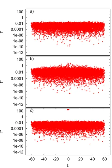
To show the reason of this behavior, we plotted the positions of the eigenvalues in theE −Γplane
for ˜κ=0.1(panel a), 1.0(panel b), 10.0(panel c) in fig. 2. As is seen in panel a), the widths do not have any energy dependence for small ˜κ. For ˜κ =1.0 we see some widths relatively large but not isolated
from others aroundE=0 in panel b). In this situation, these states with large widths may have close
0.5 0.6 0.7 0.8 0.9 1 1.1
0.01 0.1 1 10 100 κ
~
β ν
Figure 1.Fitted results ofβ, the parameter for the Brody distribution, andν, the degree of the freedom inχ2-distribution, are shown as functions of ˜κ, the
parameter controlling the coupling to the continuum. Filled squares are forβwhile filled circles are forν. The dimension of the Hamiltonian is 924, coincides with the dimension of the Hamiltonian of TBRE for
l=12 andm=6. The result is calculated from the accumulation of the 50 realizations of the random matrix.
1e-12 1e-10 1e-08 1e-06 0.0001 0.01 1 100
Γ
a)
1e-12 1e-10 1e-08 1e-06 0.0001 0.01 1 100
Γ
b)
1e-12 1e-10 1e-08 1e-06 0.0001 0.01 1 100
-60 -40 -20 0 20 40 60
Γ
E
c)
Figure 2. The positions of the complex eigenvalues in theE −Γplane for ˜κ =0.1 (a), 1.0 (b), 10.0 (c). The dimension of the Hamiltonian=924 and the plots are accumulated results of 10 realizations of the random matrix.
plane. Therefore, the reason which drive to the deviation of the width distribution from the PT one
causes also the deviation of the NNLS distribution from Wigner one, as states with large difference in
width(the imaginary axis) may have small level distance(the real axis). With further increase of ˜κto
0 0.1 0.2 0.3 0.4 0.5 0.6 0.7 0.8 0.9
0 0.5 1 1.5 2 2.5 3 3.5 4 4.5 5
P(s)
s
(a) κ=0.1κ=1.0
κ=10.0 Wigner
0 0.05 0.1 0.15 0.2 0.25
-14 -12 -10 -8 -6 -4 -2 0 2 4
P(
Γ
)
ln(Γ/<Γ>) (b)
κ=0.1 κ=1.0 κ=10.0 ν=1
Figure 3. The NNLS distribution (a) and the width distribution(b) obtained from GOE+RC model for ˜κ = 0.1(dotted line), ˜κ=1.0 (solid line), ˜κ=10.0 (dashed line) compared to the Wigner one (a) or Porter-Thomas one(b). Ω = 924, and the number of realizations is 50. For ˜κ= 0.1 and ˜κ=10.0 the results are close to the Wigner one or PT one while for ˜κ=1.0 the results are different.
1e-08 1e-06 0.0001 0.01 1 100
-20 0 20 40 60 80 100 120 140 160 Energy of Compound Nuclei
d V
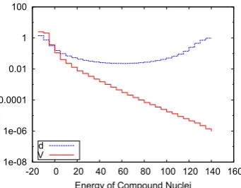
Figure 4.TheEλdependence of the size of the
coupling to the continuumVλ=Wλ2, compared with
the level spacingd. The values are the results of the averaging over an energy intervalΔE=5 and 50
realizations. In this figure, the values forEλ<, which
are not included in the effective Hamiltonian (2), are also plotted.
In fig. 3, the NNLS distribution (a) and the width distribution(b) are compared for ˜κ =
0.1,1.0,10.0 together with the simple GOE prediction, namely the Wigner one (a) or the PT one(b).
They are the combined plots for 10 realizations of the random matrix. In both ˜κ = 0.1 case and
˜
κ=10.0 case, the distributions are very close to the GOE ones, while for ˜κ=1.0 there are significant differences.
3.2 TBRE + correlated coupling model
The most significant difference of the TBRE+CC model from the GOE+RC model is the strongEλ
dependence of the couplingWλ. In fig. 4, the average of the coupling strengthW2
λover an intervalΔE and realizations is plotted as a function ofEλ. For smallκ, the coupling can be treated perturbatively,
hence the widths have the similar dependence onEf.
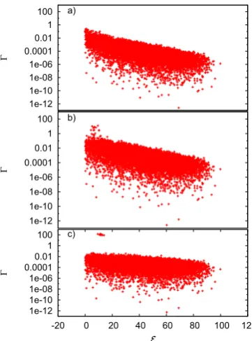
In fig. 5, positions of the complex eigenvalues are plotted on theE −Γplane for the TBRE+CC
model withl = 14 andm = 7 andκ = 0.1(panel a), 1.0(panel b) and 10.0(panel c). They are the
combined plots for 10 realizations of the random matrix. Contrary to the case of the GOE+RC model,
1e-12 1e-10 1e-08 1e-06 0.0001 0.01 1 100
Γ
a)
1e-12 1e-10 1e-08 1e-06 0.0001 0.01 1 100
Γ
b)
1e-12 1e-10 1e-08 1e-06 0.0001 0.01 1 100
-20 0 20 40 60 80 100 120
Γ
E
c)
Figure 5. The positions of the complex eigenvalues in theE −Γplane forκ =0.1 (a), 1.0 (b), 10.0 (c). The Hamiltonian is forl=14 andm=7, and the plots are accumulated results of 10 realizations.
Another difference is that the energy interval where the states with large widths deviating from
the global energy dependence forκ 1 exist is much narrower in the case of the TBRE+CC model.
(Compare the panel (b) of figs. 2 and 5.)
This strong dependence of averageΓonEf derives a completely different distribution ofΓ, as is
seen in [10], if the states all over the energy region are considered. However, in the real situation of INR, neutron widths are analyzed within very small intervals compared with the whole energy region of the excited states of nuclei. Therefore, we restricted our analysis within a small energy interval in
which the effect of the global energy dependence of the average width is, if not negligible, small.
In fig. 6, the NNLS distribution (a) and the width distribution(b) obtained from the eigenvalues in the interval 5.0≤ E ≤25.0 are compared forκ=0.1,1.0,10.0 together with the Wigner one(a) or PT one(b). Bothκ =0.1 case andκ=10.0 case, the distributions are very close to the Wigner one (a) or PT one, while forκ=1.0 there are significant difference.
In fig. 7, we plotβandνobtained from the TBRE+CC model withl=14,m=7. The analysis is
done in the energy interval 5≤ E ≤20. Although less clear than in the result of the GOE+RC model,
the deviation from the unity is seen in the intermediate region of coupling strength aroundκ1.
Such deviation is seen only in the limited energy region. In fig. 8, the dependence ofνonκ in
the different energy interval is compared. Unlike the interval 5≤ E ≤20, the behavior in the interval
0 0.1 0.2 0.3 0.4 0.5 0.6 0.7 0.8 0.9
0 0.5 1 1.5 2 2.5 3 3.5 4 4.5 5
P(s)
s
(a) κ=0.1κ=1.0
κ=10.0 Wigner
0 0.05 0.1 0.15 0.2 0.25
-14 -12 -10 -8 -6 -4 -2 0 2 4
P(
Γ
)
ln(Γ/<Γ>) (b)
κ=0.1 κ=1.0 κ=10.0 ν=1
Figure 6. The NNLS distribution (a) and the width distribution(b) obtained from the TBRE+CC model in the energy interval 5.0≤ E ≤25.0 forκ=0.1(dotted line),κ=1.0 (solid line),κ=10.0 (dot-dashed line) compared to the Wigner one (dashed line) (a) or PT one (b). l=14 andm=7, and the number of realizations is 50. For
κ= 0.1 andκ =10.0 the results are close to the Wigner one or the PT one while forκ =1.0 the results are different.
0.5 0.6 0.7 0.8 0.9 1 1.1
0.01 0.1 1 10 100 κ
β ν
Figure 7.β(square) andν(circle) obtained from the result of the TBRE+CC model withl=14,m=7. States in the energy interval 5≤ E ≤20 are considered. The number of realizations is 50.
0.5 0.6 0.7 0.8 0.9 1 1.1
0.01 0.1 1 10 100 κ
5-20 20-35 35-50
Figure 8.νobtained from the TBRE+CC model with
4 Conclusion
Motivated by the recent claim that the neutron resonance width distribution does not support the random matrix theory, we examine the consequence of the super-radiant mechanism in the strong
continuum coupling and the effect of the correlation between the target and the compound nuclei
on the statistics of both the levels and the widths simultaneously, by controlling the strength to the continuum.
If the coupling to the continuum is large, several states have relatively large widths, resulting the deviation from the GOE limit both in the nearest neighbor level spacing distribution and the width distribution. However in the limit of strong coupling, the behaviors of both levels and widths are restored to the GOE ones, because only one state monopolizes the coupling to the continuum in this limit, and the rest states have the normal statistical property.
The effect of the correlation between the target and the compound states results in the global
excitation energy dependence of the widths. Therefore, the width distribution for whole spectrum
is completely different from the GOE one. However, if the width distribution is evaluated within a
relatively narrow energy interval, it approximately follows the Porter-Thomas distribution as long as the coupling to the continuum is week.
When the coupling to the continuum becomes large, both the NNLS distribution and the width distribution deviate from the ones of the GOE in the energy interval where the states with large widths crowd. However, in other energy intervals away from "width concentrating region", the distributions are similar to the GOE ones. With further increase of the strength, both the NNLS distribution and the width distribution come again close to the GOE ones.
The deviation of the width distribution from the Porter-Thomas one and the deviation of the NNLS distribution from the Wigner one occur coincidently within the model we adopted.
References
[1] N. Bohr, Science137, 344 (1936)
[2] C.E. Porter,Statistical Theories of Spectra: Fluctuations(Academic, New York, 1965)
[3] R. U. Haq, A. Pandey, and O. Bohigas, Phys. Rev. Lett.48, 1086 (1982)
O. Bohigas, R. U. Haq, and A. Pandey,Nuclear Data for Science and Technology (Reidel,
Dor-drecht, 1983) 809
[4] P. E. Koehler et al, Phys. Rev. Lett.105, 072592 (2010)
[5] P. E. Koehler, Phys.Rev. C84, 034312 (2011)
[6] J. F. Shriner Jr, H. A. Weidenmüller, and G. E. Mitchell, arXiv:1209.2439v3 (2014)
[7] E. G. Reich, Nature,466, 1032 (2010)
[8] H.A. Weidenmüller, Phys. Rev. Lett.105, 232501(2010)
[9] G. L. Celardo, N. Auerbach, F. M. Izrailev, and V. G. Zelevinsky, Phys. Rev. Lett. 106,
042501(2011)
[10] A. Volya, Phys. Rev. C83, 044312(2011)
[11] S. Mizutori and V. G. Zelevinsky, Zeit. für Phys. A346, 1(1993)
[12] H. Feshbach, Ann. Phys. (NY)5, 357(1958)
C. Mahaux and H. A. Weidenmüller,Shell-model approach to nuclear reactions(North Holland,