Simulations of Ionospheric Behavior Driven by HF Radio Waves
at the Initial Stage
Jing Chen1, 2, Qingliang Li2, Yubo Yan2, Haiqin Che2, Guanglin Ma2, and Guang Yuan1, *
Abstract—This study explores the variability in the electric field, plasma number density, and plasma velocity driven by high-frequency (HF) radio wave injected into the vertically stratified ionosphere at a millisecond time scale after switch-on of the radio transmitter. It was found that the mode conversion process of electromagnetic (EM) waves took place at the reflection heights of both the R-X (right-circularly polarized extraordinary wave, R-X) and L-O (left-(right-circularly polarized ordinary wave, L-O) modes. The ionospheric electron number density was remarkably oscillatory. A depletion of ionospheric ion number density at the L-O mode turning point and two ion number density peaks on each side of the O-mode reflection region were discovered. The turbulent layer of the ion density peak at the bottom of the critical height shifted downwards, which qualitatively conforms to the observations made at the Arecibo and the EISCAT. The vertical electron velocity oscillated near the L-O mode reflection point. The vertical ion velocity remained positive above the reflection height of the L-O mode and remained negative below this height. These results, which were derived using realistic length scales, ion masses, pump waves, and other plasma parameters, are consistent with theoretical predictions and prior experimental observations, and should thus be useful for understanding the linear and nonlinear interactions between the HF EM wave and the ionospheric plasma at the initial stage.
1. INTRODUCTION
The ionosphere is a natural plasma laboratory, and as such, it is of significant interest both from geophysical perspectives and plasma physics [1]. Therefore, many different scientific and technological objectives have motivated the ionospheric modification using high-power and high-frequency (HF) transmitters [2–4]. A considerable number of active ionospheric experiments designed to investigate the F-region artificial ionospheric turbulence, including large-scale electron and ion temperature and density perturbations [5, 6], artificial field-aligned irregularities [7, 8], stimulated electromagnetic emissions [9– 11], and Langmuir turbulence [12] have been performed. To explain the observed phenomena, studies of the associated physical mechanisms, such as ohmic absorption, oscillating two-stream instability, and parametric instability, have been developing rapidly [13–15]. A high-power radio wave can excite the particular wave modes and enhance plasma turbulence, which in turn causes the anomalous plasma heating [16–18]. It has been recognized that wave-wave interactions determine the characteristics of F-region modifications to a large extent [19]. As the primary mechanism of turbulence excitation, the parametric decay instability (PDI) involves the conversion of HF electromagnetic (EM) waves into Langmuir waves and ion-acoustic waves, which could lead to the development of solitons and the Langmuir cavitons under the existence of the vertical density gradient in the F-region [20–22].
Received 11 May 2019, Accepted 18 August 2019, Scheduled 3 September 2019
* Corresponding author: Guang Yuan ([email protected]).
1 Optics and Optoelectronics Laboratory, Department of Physics, Ocean University of China, Qingdao 266100, China. 2 National
One of the important features of the PDI caused by the nonlinear effects of wave and plasma interactions is that there is a limited electric field threshold [23–25]. High-frequency pump waves excite a noticeable standing wave pattern at the reflection points of ordinary wave (O-mode). The electric field strength of standing waves will then increase dramatically, and this is called the “swelling” of the electric field. When this electric-field amplitude of the standing wave exceeds the limited electric field threshold, other instabilities (i.e., Langmuir decay instability and oscillating two-stream instabilities) can be induced. Therefore, it is necessary to accurately calculate the variation within electric fields, plasma densities, and other parameters during the initial process in the reflection area. However, parametric instabilities are excited within a few milliseconds after a radio transmitter is activated [26, 27]. For instance, the EISCAT heating experiments showed the enhanced ion-lines induced by PDI within the initial 100 ms of heating [28], and the HF-induced small-scale plasma depletions have been detected instantly within 5 ms at the Arecibo [29]. Nevertheless, these observations provide very limited insights into the physical processes occurring within PDI over such short time intervals. Thus, numerical simulations are essential for studying the interactions between EM waves and plasma, and simulation results are of great benefit for understanding the physical phenomena that are difficult to observe by artificial ionospheric modification experiments at the millisecond time scale.
In recent decades, numerical simulation methods rather than purely numerical analyses of ionospheric heating have been shown to provide effective measures for understanding the interactions between ionospheric plasma and EM waves because the excitation and the development of parametric instabilities can be visualized by the simulations [30–32]. To better simulate this complex, nonlinear, and impulsive interactions in a natural way, it is critical to accurately describe the physical model and avoid distortions caused by numerical errors. The difficulty of simulating the parametric instabilities process is the accurate description of physical parameters enabling variation in the geomagnetic field, temperature characteristic, electromagnetic field and plasma collision frequency at different positions. The original finite difference time domain (FDTD) method, as a standard technique for numerically solving Maxwell’s equations, is considered a primary alternative to simulating PDI because the physical model involves Maxwell’s equations [33]. Additionally, the grid-based FDTD structures of Yee (1966) allow material properties (such as temperature, topography, and electron density) to be defined separately at each point [34]. Thus, this method can handle complex, nonlinear, and impulsive interactions between HF waves and the plasma in a natural way [35]. However, the original FDTD method lacks temporal and spatial discretization and is absence of the time advancement scheme of other physical quantities, such as plasma number density and velocity involved in simulating the PDI process. Hence, the classical FDTD method is insufficient for simulating this process. A few improved FDTD models described the radio waves propagation in plasma have been reported [36, 37]. More importantly, Young (1994) arranged plasma fluid velocity vector and electric field vector in same Yee grid in order to couple between the Maxwell equations and Euler equation [38]. Yu and Simpson (2010) developed a new three-dimensional FDTD model to simulate EM wave propagation in the anisotropic magnetized cold plasma by letting the current density and electric field share the same nodes [39]. Therefore, the schemes based on the FDTD method can feasibly simulate the variability in ionospheric parameters during the EM wave-driven ionospheric perturbation process. In this study, we investigate the variation in the electric field, plasma density, and plasma velocity driven by HF radio waves at the millisecond time scale according to plasma two-fluid theory and via numerical simulations based on an advanced FDTD method which improved the spatial and temporal arrangements and the time advancement scheme for the above-mentioned physical quantities. Such simulations, involving realistic scales of the ionosphere and wavelengths of the EM waves, are of great benefit for understanding the physical mechanisms of artificial ionospheric modification experiments.
2. METHODOLOGY
2.1. Physical and Mathematical Model
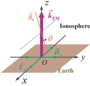
Figure 1. Schematic showing the simulation model of the electromagnetic (EM) wave propagation in ionosphere: B0 is the geomagnetic field;kEM is the propagation direction of the injected EM wave;Ex andHy are the initial polarized direction of the electricfield and magnetic field of the injected EM wave,
respectively.
in the x-z plane. It is necessary to define the geomagnetic field, which is of great importance to the plasma dynamics in F-region where collision frequencies between particles are low, because the motions of charged particles are influenced by the magnetic field [19].
The plasma component species in this simulation model of ionosphere were electrons and oxygen ions O+. O+ was considered as the major ionic component in F-region because the number of the O+ ions is higher than that of other ions, such as NO+ and O+
2 [40, 41]. The plasma two-fluid theory was adopted to mathematically describe the ionospheric behavior driven by the EM waves propagation in the ionospheric plasma. The plasma two-fluid theory is essentially a macroscopic theory based on fluid equations of mass as well as charge, momentum and energy continuity together with the Maxwell equations. Because the ∂Tα/∂tduring 5 milliseconds is small enough that such the energy equation is
not indeed calculated. Therefore, there are four equations to describe the initial ionospheric behavior. The magnetized plasma governing equations from this theory were cast in terms of Maxwell’s equations (Eqs. (1)–(2)) coupled to the continuity equation (Eq. (4)) and the momentum equation (Eq. (4)). These equations can be expressed as follows:
−μ0∂
H
∂t = ∇ ×E; (1)
−ε0∂
E
∂t = ∇ ×H−
α
NαqαUα; (2)
∂Nα
∂t = −∇ ·(NαUα); (3)
NαmαdUα
dt = Nαqα[E+ Uα×(B0+ B)]−NαmαναUα− ∇(kBNαTα), (4) whereαrepresents the electron eor oxygen ioni, andx,y, andz are the unit vectors in thex-,y-, and z-directions, respectively. H =Hx+Hy+Hzand E =Ex+Ey+Ezare the magnetic field and the electric
field perturbation, respectively. UαandNα are the time-varying velocity and the number density of the
plasma fluid, respectively. Tα signifies the electron or O+ temperature. ε0, μ0 and kB are the vacuum permittivity, permeability and Boltzmann’s constant, respectively. Here, να and mα are the particle collision frequency and mass, respectively. Additionally,qi =eandqe =−erepresent charge magnitude of the ion and the electron, respectively. It should be noted that the dUα/dt ≡∂Uα/∂t+ (Uα· ∇)Uα is the convective derivative in which (Uα· ∇) is a scalar differential operator.
during the millisecond ionospheric heating [27]. As a result, only the vertical gradient of variations was considered and the transverse variations were negligible in this model. Notice that the variation of kBNα(∂Tα/∂z), a part of the last term in right-hand side in Eq. (4), has negligible influence on Eq. (4)
at a millisecond time scale. Hence, the electron and ion temperature in this model at a millisecond time scale were set to be constant when simulating the initial variations.
Based on this physical model, the developed FDTD scheme was applied to simulate the nonlinear interactions between HF waves and the ionospheric plasma through a complete spatial and temporal discretization scheme and the time-advancement equations for plasma number density and plasma velocity.
2.2. Numerical Setup
The initial conditions of the simulation parameters relevant to experiments at the EISCAT facility are shown in Table 1. The simulated altitude ranged from 190 km to 340 km. We assumed the switched
Table 1. Physical simulation parameters.
Parameter Value
Simulation range 190–340 km
Simulation time 0.667–6.667 ms
Switched work
time of transmitter 0 ms
Density profile N0(z) = 2.5×10¹¹exp[−(z−300×103)2/109] Geomagnetic field
using EISCATa B0=4.8×10⁻⁵[xsin(12◦)−zcos(12◦)]
Electron/ion temperature 1500 K
Electron collision frequency νe=400 s−1
Ion collision frequency νO+=300 s−1
Pump wave
Frequency 4.03 MHz
Wavelength 74.37 m
Maximum amplitude 1.5 V/m
Pulse type sine
Polarization time-varying linearly polarized
Ex(t)= 1.5 sin(ω0t)
Injected height 200 km
Theoretical critical
altitude of X mode 274.99 km
Theoretical critical
altitude of O mode 285.16 km
Δz 2.48 m
Δt 4.13×10⁻⁹s
Number of time steps 1,451,142
all-simulation Time sampling resolution/
Frequency resolution 750Δt= 3.101×10
−3ms/0.322 MHz
from 1.02 ms to 1.12 ms
Time sampling resolution/
Frequency resolution 10Δt= 4.135×10
−5ms/24.184 MHz
work time of transmitter was 0 ms. The simulation began att= 0.667 ms, because the altitude of EM wave source was set to be 200 km. The simulation time was fromt= 0.667 ms to t= 6.667 ms.
According to the peak electron density Nmax = 2.5 × 10¹¹m−3, the peak plasma frequency
f0F2=21π
Neqe2
meε0=4.489 MHz can be calculated. Thus, the incident wave frequency was f0 = 4.03 MHz
(w0 = 2.53×10⁷s−1), which is lower than the peak plasma frequency. According to the A-H equation, the theoretical altitude of the X-mode and O-mode for the incident wave were hX = 274.99 km and hO = 285.16 km, respectively. The cutoff of the O-mode is above the cutoff of the X-mode. The electric-and magnetic-field of the injected linearly polarized wave, which was a sinusoidal amplitude modulation wave, were set to Ex(t) = 1.5 sin(ω0t) and Hy(t) = Ex(t)/c/μ0. Other electric- and magnetic-field components were set to zero.
The geomagnetic field, B0= 4.8×10⁻⁵[xsin(12◦) − zcos(12◦)] T, was selected, which was in accordance with the EISCAT geomagnetic field. The electron and ion temperatures were set to 1500 K. Because the major ionic component was O+, the ion mass was set to mO+ = 16mp, where mp = 1836,
me is the proton mass, andme= 9.1×10⁻³¹kg is the electron mass.
Appropriate spatial grid sizes and temporal steps chosen from the initial conditions can maintain the stability of the simulation. In an unstable simulation, small numerical artifacts may cause errors that rapidly grow with time, to the extent of altering or overwhelming the simulation results [35]. In
order to satisfy the Courant-Friedrichs-Lewy conditioncΔt≤[1−(ωpΔt/2)2]/
1/Δz2 [42], the fixed spatial grid length, Δz=λ/30 = 2.48 m, was determined by the incident wavelength and fixed temporal step was set to Δt= Δz/2c= 4.13×10⁻⁹s.
3. SIMULATION RESULTS
3.1. Full-Scale Simulations of Ionospheric Behavior
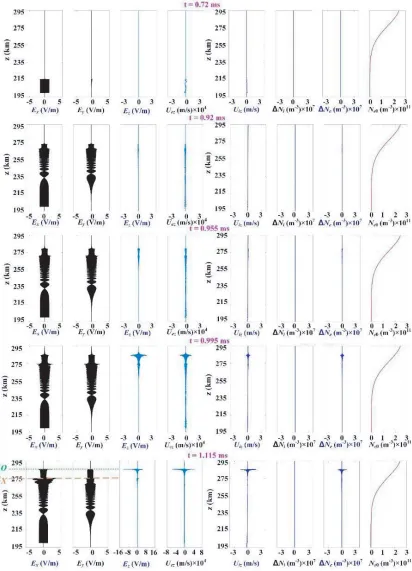
Typically, full-scale results of fluctuations in the electric field, plasma velocity, and plasma density are shown in Figures 2 and 3. The development processes modified by the HF EM waves can be divided into those of electric field swelling and the enhancement of plasma turbulence.
Figure 2 shows the variation of physical parameters during the process of electric field swelling. Before a pump wave reaches the O-mode reflection point, the electric field in the x direction Ex
propagates upward and maintains the sinusoidal wave shape. This phenomenon can validate the propagation model of EM wave. Meanwhile, the linearly polarized incident wave undergoes Faraday rotation and splits. Hence, Ey have been excited, as can be seen at t= 0.72 ms and t= 0.92 ms.
It is obvious that the X- and O-modes both have cutoffs (turning points) att= 0.955 ms. According to the A-H equation, the theoretical reflection heights of the X-mode and O-mode arehX = 274.99 km and hO = 285.16 km, respectively. In our simulation, the altitudes of the X-mode and O-mode were hX = 274.90 km and hO = 285.23 km, respectively. The errors for the reflection heights of the X-mode and O-mode were within an acceptable error range. Hence, the simulation results for the turning point corresponded well with the theoretical predictions. The EM waves arrived at the cutoffs of the X-mode and O-mode att= 0.917 ms and t= 0.951 ms, respectively.
Ez at the O-mode turning points exhibited obvious swelling, while that at the reflection point of
the X-mode exhibited no significant change, as shown att= 0.995 ms. Hence, the electric field strength of the standing wave pattern grew at the reflection point of the X-mode, but its swelling was much weaker than at that of the O-mode wave. At t= 1.115 ms, the Ez was raised up to 16 V/m near the altitudes of the O-mode hO because the EM wave underwent mode conversion to a large-amplitude electrostatic wave, which could lead to the development of strong Langmuir turbulence [20]. Therefore, the electric field of each direction changed most obviously near the reflection points when compared with other regions.
At t = 1.12 ms, the electron vertical velocity on the order of 104 at hO was affected by the propagation of EM waves, and the ion vertical velocity on the order of 100 changed slightly due to the ion:electron mass ratio equaling 29376. The electron density exhibited significant variation nearhO, which was closely related to the electric field, especially Ez. However, the ion density was remarkably
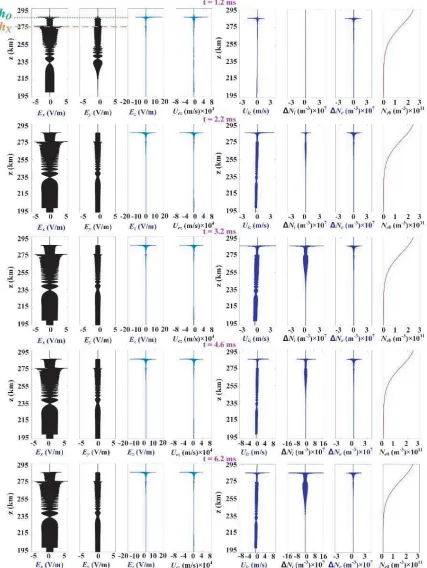
After t= 1.2 ms, it was found that the amplitudes of Ex and Ey at hX were greater than those at hO, which demonstrates that the energy in x- and y-directions on the X-mode critical point are
higher than that on the O-mode critical point. From 1.2 ms to 6.2 ms, it was obvious that Ez at hO
maintained a relatively stable, large-amplitude oscillation, which was close to 20 V/m. Meanwhile, the vertical electron velocity Uez at hO continued to oscillate, which means the electrons near the O-mode
reflection point migrated upward or downward. In all regions, the vertical ion velocityUiz had non-zero
values, which can be explained by ions in the simulated ionosphere being affected by the propagation of HF EM waves. The noticeable maximum of the electron and ion density fluctuations were at the O-mode reflection point. The variations in density reached up to 7 orders of magnitude.
3.2. Mode Conversion of Electric Field
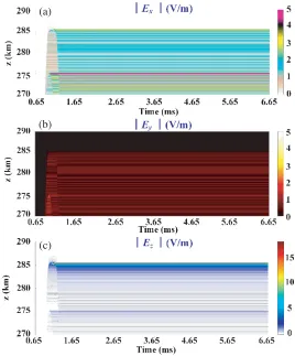
To clearly present the variation in the electric field at the reflection region, the electric field from 270 km to 290 km was extracted between 0.65 ms and 6.65 ms (Figure 4). It is notable that the amplitudes ofEx
andEy athX were larger than athO. The maxima ofExand Ey at hX both exceeded 3 V/m. Swelling
of the Ez amplitude could be generated at hO and at hX, which indicates that parametric instability
was excited both at the X-mode and O-mode turning points. However, the swelling of theEz amplitude
at hO was greater than athX. The maximum of Ez at hO exceed 16 V/m. Therefore, the pump electric
fieldEx at hX and the excited electric field Ez at hO exhibited the most obvious changes.
(a)
(b)
(c)
Figure 4. Simulations of the spatial evolution of the electric field in the: (a) x-, (b) y-, and (c) z-directions from 0.65 to 6.65 ms.
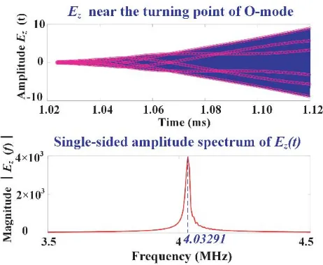
To investigate the frequency matching conditions of the PDI,Ez near hO from 1.02 ms to 1.12 ms
were extracted. The frequency spectrum of the Ez is shown in Figure 5. The frequencyEz at hO was
Figure 5. Frequency spectra ofEznear the turning points of the O-mode using data from 1.02–1.12 ms.
conditions of the PDI, ω0 = ωI+ωL, where ωI and ωL are the angular frequency of the ion-acoustic waves and the Langmuir waves, respectively. The frequency of ion-acoustic waves was∼1.96 kHz. The frequency of the ion-acoustic wave can range from a few kHz to tens of kHz. For instance, experimental observations revealed a ∼ 4 kHz frequency for ion-acoustic waves [43] at the Arecibo and 5 kHz at EISCAT [28].
Figure 6 presents the spectral energy density Wk(ω, k) = ΔE2/Δk obtained by calculating the
spatial Fourier transform of Ez from 283.707 km to 285.690 km with w fixed at the frequency of the
incident wave (4.03 MHz), where Δk is the differential wavenumber, and ΔE2 denotes the differential squared electric field. It can be seen that the energy was concentrated at a wave number of 0, which represents the pump wave because the wave length of the pump (74.37 m) is larger than that of other waves. Such large amounts of energy may cause thermal electrons and electron acceleration in the presence of Langmuir waves on the O-mode critical layer. The other waves could not be observed because this method did not include the ponderomotive force, which will be the focus of future work.
3.3. Variation in Plasma Velocity
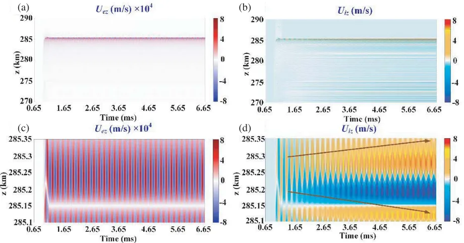
To predict the behavior of plasma movements, the plasma velocity in the z-direction is of particular concern and can be used to infer upward or downward motions. These movements lead to variations in the vertically stratified ionosphere, which can be mirrored on the incoherent radial observations of the spectral features known as cascades, collapses, and outshifted plasma lines [44]. The evolutions of Uiz
and Uez are presented in Figure 7, which reveals that the electron and ion velocities were on the order of 104 and 100, respectively, and were affected by the propagation of EM waves. The amplitude of the plasma vertical velocity at the reflection point of the O-mode was larger than in other regions.
(c) (d)
(a) (b)
Figure 7. Simulations of the temporal evolution of the plasma velocity near the O and X-mode turning point for: (a) Uez and (b)Uiz, and magnifications of these patterns through the condensing of z (km), (c)Uez and (d)Uiz.
Closeups of the region of the O-mode turning point are displayed in Figures 7(c) and (d). It is notable that Uez is either positive or negative with turbulence near the O-mode turning point, which implies that the electrons are oscillating. It is also noteworthy that the oscillation frequency of Uez is high near the O-mode turning point, which suggests that the electrons here oscillate rapidly. Hence, the variation of electrons over a fast time scale can be observed with difficultly, and the change of electrons on the slow time scale can be traced by the movement of ions because the ambipolar electrostatic force makes both electrons and ions move in phase with the ion-acoustic waves.
It was found that the ion velocity was lower than the electron velocity by approximately four orders of magnitude, which indicates that the amount of electron movement can be separated into HFs and slow time scales, and that ions are stationary at HF scales. At the turning point of the O-mode, Uiz
remains positive above the reflection height and remains negative below the reflection height. This will lead to enhanced diffusion and the subsequent movement of ions away from the region of interaction.
3.4. Change of Plasma Density
(a) (b)
(c) (d)
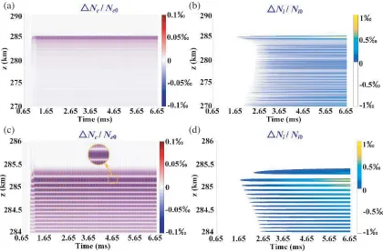
Figure 8. Simulations of the temporal evolution of the plasma density near the L-O mode turning point, where ΔNe is the electron density fluctuation; Ne is the initial electron density; ΔNi is the fluctuation in the electron density, andNi is the initial electron density: (a) ΔNe/Ne, (b) ΔNi/Ni, and magnifications of these patterns through the compressing ofz (km), (c) ΔNe/Ne0 and (d) ΔNi/Ni.
Closeups of the region at the O-mode reflection height are displayed in Figures 8(c) and (d). Figure 8(c) indicates that the electron density fluctuation ΔNe oscillated rapidly on the fast time scale. The reason is that the electrons could instantly respond to the HF waves due to their small mass.
The ambipolar electrostatic force causes both electrons and ions to move in phase with the ion-acoustic waves [45]. Hence, the movement of electrons on the slow time scale can be traced by the movement of ions. The change in ion density near O-mode reflection region is presented in Figure 8(d). After t = 2.5 ms, a valley of ionospheric ion number density at the L-O mode turning point and two ion density peaks on each side of the O-mode reflection region are observed. After t = 5.65 ms, the scope of the ion density peak below the cutoff altitude extends downward. The ion density fluctuation within milliseconds is on the magnitude of 1 ; however, it is on the order of 107m−3 in quantity, which can manifest the ion motion away from the O-mode reflection region and accumulation on each side of this region. And the turbulent layer of ion density peak at the bottom of the O-mode critical height was shifted downward, which suggests that the EM wave could be reflected at a lower height below the initial reflection point, and the process will then be repeated at the new reflection height. Therefore, the enhanced ion- and plasma-lines of experimental observations descend sequentially in altitude, which has been observed at both the Arecibo [46] and EISCAT [47] during heating experiments.
4. CONCLUSIONS
the electric field strength of the standing wave pattern at the reflection point of the X-mode grew, but its swelling effect was much weaker than that of the O-mode wave. The vertical ion velocity remained positive above the L-O mode turning point and remained negative below this refection height. The ionospheric electron number density rapidly oscillated with the small-scale HF electric field near the L-O mode reflection region. The ion density depletion created at the L-O mode turning point and two ion density peaks formed on each side of this reflection region were observed. This turbulent layer of the ion density peak at the bottom of the O-mode critical height was shifted downward, which is consistent with the observations made at both the Arecibo and at EISCAT. Future extensions of this work may consider the effects on parametric instability in the ionosphere due to the presence of different ponderomotive forces and the exciting condition in the governing equation, allowing for the improvement of the kinetic model of plasma dynamics. The scheme will be developed to extend the model to more complex situations and to more than one dimension in space.
ACKNOWLEDGMENT
We are grateful to Haiying Li, Shucan Ge, Jingfan Gao, Musong Cheng, Cheng Wang, Wen Yi, Ting Zhu and Moran Liu for their selfless assistance, and we would like to thank everyone who has contributed to this work.
Funding: This work was supported by the National Natural Science Foundation of China [Grant No. 41476082], the Innovation Foundation of the China Electronics Technology Group Corporation [Grant No. KJ1602004), and the Foundation of the National Key Laboratory of Electromagnetic Environment of China Electronics Technology Group Corporation [Grant No. 201803001].
REFERENCES
1. Kelley, M. C., The Earth’s Ionosphere: Plasma Physics and Electrodynamics, Vol. 96, Academic Press, 2009.
2. Bernhardt, P., W. A. Scales, S. Grach, A. Keroshtin, D. Kotik, and S. Polyakov, “Excitation of artificial airglow by high power radio waves from the “Sura” ionospheric heating facility,”Geophys. Res. Lett., Vol. 18, 1477–1480, 1991.
3. Carroll, J., E. Violette, and W. Utlaut, “The Platteville high power facility,” Radio Sci., Vol. 9, 889–894, 1974.
4. Kuo, S. and A. Snyder, “Artificial plasma cusp generated by upper hybrid instabilities in HF heating experiments at HAARP,”J. Geophys. Res. — Space Phys., Vol. 118, 2734–2743, 2013. 5. Robinson, T., F. Honary, A. Stocker, T. Jones, and P. Stubbe, “First EISCAT observations of the
modification of F-region electron temperatures during RF heating at harmonics of the electron gyro frequency,”Journal of Atmospheric and Terrestrial Physics, Vol. 58, 385–395, 1996.
6. Wu, J., J. Wu, and Z. Xu, “Results of ionospheric heating experiments involving an enhancement in electron density in the high latitude ionosphere,” Plasma Sci. Technol., Vol. 18, 890, 2016. 7. Blagoveshchenskaya, N., T. Borisova, V. Kornienko, V. Frolov, M. Rietveld, and A. Brekke, “Some
distinctive features in the behavior of small-scale artificial ionospheric irregularities at mid-and high latitudes,” Radiophys. Quantum Electron., Vol. 50, 619–632, 2007.
8. Pedersen, T., M. McCarrick, B. Reinisch, B. Watkins, R. Hamel, and V. Paznukhov, “Production of artificial ionospheric layers by frequency sweeping near the 2nd gyroharmonic,” Ann. Geophys., Vol. 29, 2011.
9. Kosch, M., T. Pedersen, M. Rietveld, B. Gustavsson, S. Grach, and T. Hagfors, “Artificial optical emissions in the high-latitude thermosphere induced by powerful radio waves: An observational review,”Adv. Space Res., Vol. 40, 365–376, 2007.
10. Leyser, T., “Stimulated electromagnetic emissions by high-frequency electromagnetic pumping of the ionospheric plasma,” Space Sci. Rev., Vol. 98, 223–328, 2001.
12. Stubbe, P., H. Kohl, and M. Rietveld, “Langmuir turbulence and ionospheric modification,” J. Geophys. Res. — Space Phys., Vol. 97, 6285–6297, 1992.
13. Gurevich, A. V., “Nonlinear effects in the ionosphere,”Phys. Usp., Vol. 50, 1091–1121, 2007. 14. Huang, J. and S. Kuo, “Cyclotron harmonic effect on the thermal oscillating two-stream instability
in the high latitude ionosphere,”J. Geophys. Res. — Space Phys., Vol. 99, 2173–2181, 1994. 15. Kuo, S., M. Lee, and P. Kossey, “Excitation of oscillating two stream instability by upper hybrid
pump waves in ionospheric heating experiments at Tromso,” Geophys. Res. Lett., Vol. 24, 2969– 2972, 1997.
16. Robinson, T., A. Stocker, G. Bond, P. Eglitis, D. Wright, T. Jones, et al., “First CUTLASS-EISCAT heating results,”Adv. Space Res., Vol. 21, 663–666, 1998.
17. Djuth, F., P. Stubbe, M. Sulzer, H. Kohl, M. Rietveld, and J. Elder, “Altitude characteristics of plasma turbulence excited with the Tromsø superheater,”J. Geophys. Res. — Space Phys., Vol. 99, 333–339, 1994.
18. Wong, A., J. Santoru, and G. Sivjee, “Active stimulation of the auroral plasma,”J. Geophys. Res. — Space Phys., Vol. 86, 7718–7732, 1981.
19. Robinson, T., “The heating of the high lattitude ionosphere by high power radio waves,” Physics Reports, Vol. 179, 79–209, 1989.
20. DuBois, D. F., H. A. Rose, and D. Russell, “Excitation of strong Langmuir turbulence in plasmas near critical density: Application to HF heating of the ionosphere,” J. Geophys. Res. — Space Phys., Vol. 95, 21221–21272, 1990.
21. Frolov, V., L. Erukhimov, S. Metelev, and E. Sergeev, “Temporal behaviour of artificial small-scale ionospheric irregularities: Review of experimental results,” J. Atmos. Sol.-Terr. Phys., Vol. 59, 2317–2333, 1997.
22. Wong, A., T. Tanikawa, and A. Kuthi, “Observation of ionospheric cavitons,” Physical Review Letters, Vol. 58, 1375, 1987.
23. Vas’ kov, V. and N. Ryabova, “Parametric excitation of high frequency plasma oscillations in the ionosphere by a powerful extraordinary radio wave,”Adv. Space Res., Vol. 21, 697–700, 1998. 24. Pandey, R. S. and D. Singh, “Study of electromagnetic ion-cyclotron instability in a
magnetoplasma,” Progress In Electromagnetics Research, Vol. 14, 147–161, 2010.
25. Xiang, W., Z. Chen, M. Liu, F. Honary, B. Ni, and Z. Zhao, “Threshold of parametric instability in the ionospheric heating experiments,”Plasma Sci. Technol., Vol. 20, 115301, 2018.
26. Duncan, L. and J. Sheerin, “High-resolution studies of the HF ionospheric modification interaction region,” J. Geophys. Res. — Space Phys., Vol. 90, 8371–8376, 1985.
27. Eliasson, B. and L. Stenflo, “Full-scale simulation study of stimulated electromagnetic emissions: The first ten milliseconds,”J. Plasma Phys., Vol. 76, 369–375, 2010.
28. Djuth, F., B. Isham, M. Rietveld, T. Hagfors, and C. La Hoz, “First 100 ms of HF modification at Tromsø, Norway,” J. Geophys. Res. — Space Phys., Vol. 109, 2004.
29. Isham, B., W. Birkmayer, T. Hagfors, and W. Kofman, “Observations of small-scale plasma density depletions in Arecibo HF heating experiments,” J. Geophys. Res. — Space Phys., Vol. 92, 4629– 4637, 1987.
30. Cros, B., J. Godiot, G. Matthieussent, and A. H´eron, “Laboratory simulation of ionospheric heating experiment,” Geophys. Res. Lett., Vol. 18, 1623–1626, 1991.
31. Eliasson, B., X. Shao, G. Milikh, E. V. Mishin, and K. Papadopoulos, “Numerical modeling of artificial ionospheric layers driven by high-power HF heating,” J. Geophys. Res. — Space Phys., Vol. 117, 2012.
32. Goodman, S., H. Usui, and H. Matsumoto, “Particle-in-cell (PIC) simulations of electromagnetic emissions from plasma turbulence,”Phys. Plasmas, Vol. 1, 1765–1767, 1994.
34. Simpson, J. J., “On the possibility of high-level transient coronal mass ejection — induced ionospheric current coupling to electric power grids,” J. Geophys. Res. — Space Phys., Vol. 116, 2011.
35. Cummer, S. A., “An analysis of new and existing FDTD methods for isotropic cold plasma and a method for improving their accuracy,” IEEE Trans. Antennas Propag., Vol. 45, 392–400, 1997. 36. Wang, M.-Y., J. Xu, J. Wu, B. Wei, H.-L. Li, T. Xu, and D.-B. Ge, “FDTD study on
wave propagation in layered structures with biaxial anisotropic metamaterials,” Progress In Electromagnetics Research, Vol. 81, 253–265, 2008.
37. Simpson, J. J. and A. Taflove, “A review of progress in FDTD Maxwell’s equations modeling of impulsive subionospheric propagation below 300 kHz,” IEEE Trans. Antennas Propag., Vol. 55, 1582–1590, 2007.
38. Young, J., “A full finite difference time domain implementation for radio wave propagation in a plasma,”Radio Sci., Vol. 29, 1513–1522, 1994.
39. Yu, Y. and J. J. Simpson, “An EJ collocated 3-D FDTD model of electromagnetic wave propagation in magnetized cold plasma,”IEEE Trans. Antennas Propag., Vol. 58, 469–478, 2010.
40. Blaunstein, N. and E. Plohotniuc, Ionosphere and Applied Aspects of Radio Communication and Radar, CRC Press, 2008.
41. Rawer, K., Wave Propagation in the Ionosphere, Vol. 5, Springer Science & Business Media, 2013. 42. Fletcher, C. A., “Computational galerkin methods,” Computational Galerkin Methods, Springer,
Berlin, 1984.
43. Carlson, H. C., W. E. Gordon, and R. L. Showen, “High frequency induced enhancements of the incoherent scatter spectrum at Arecibo,” Journal of Geophysical Research, Vol. 77, 1242–1250, 1972.
44. Depierreux, S., C. Labaune, J. Fuchs, D. Pesme, V. Tikhonchuk, and H. Baldis, “Langmuir decay instability cascade in laser-plasma experiments,” Physical Review Letters, Vol. 89, 045001, 2002. 45. Bryers, C., M. Kosch, A. Senior, M. Rietveld, and T. Yeoman, “The thresholds of ionospheric
plasma instabilities pumped by high-frequency radio waves at EISCAT,”J. Geophys. Res. — Space Phys., Vol. 118, 7472–7481, 2013.
46. Bernhardt, P., C. Tepley, and L. Duncan, “Airglow enhancements associated with plasma cavities formed during ionospheric heating experiments,” J. Geophys. Res. — Space Phys., Vol. 94, 9071– 9092, 1989.