DETERMINING THE SPECIFIC GROUND
CONDUCTIVITY AIDED BY THE HORIZONTAL ELECTRIC DIPOLE ANTENNA NEAR THE GROUND SURFACE
S. V. A. Makki
Department of Electrical Engineering Engineering Faculty
Razi University
Tagh-e-Bostan, Kermanshah, 67149, Iran
T. Z. Ershadi and M. S. Abrishamian
Electrical Faculty
KHaje Nasir Toosi University
Seyed KHandan Bridge, Tehran, 16315, Iran
1. INTRODUCTION
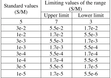
Determining the transmitter’s Field Strength (FS) is influ-enced by Ground Conductivity (GC) especially in Medium Wave (FS>60 dBµV/M) [1]. In the aforementioned band and regarding the related recommendations [2] the GC is defined in 9 intervals (Table 1).
Table 1. Standard values and ranges of GC.
Limiting values of the range (S/M)
Lower limit Upper limit
Standard values (S/M)
3 7
5
1.7e-2 5.5e-2
3e-2
5.5e-3 1.7e-2
1e-2
1.7e-3 5.5e-3
3e-3
5.5e-4 1.7e-3
1e-3
1.7e-4 5.5e-4
3e-4
5.5e-5 1.7e-4
1e-4
1.7e-5 5.5e-5
3e-5
5.5e-6 1.7e-5
1e-5
The conductivity and permittivity effect on the environment’s propagation constant, which itself determines the field structure and propagation path attenuation, is in a way that conductivity is the most dependent. For example in the Fig. 1 the propagation constant (K2) has been drawn in three frequencies 0.5, 1 & 1.5 MHz based on the permittivity (up) and conductivity (down). It is obvious that the propagation constant is not sensitive to permittivity changes, but fully dependent on conductivity.
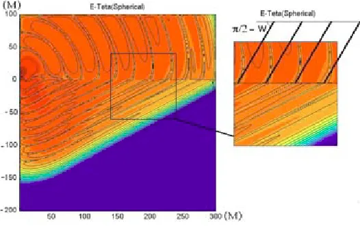
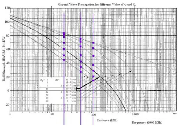
The related permittivity is considered regarding previous figures and after determining the GC. The simulated electric field by Finite Difference Time Domain (FDTD) is drawn in Fig. 2. The tilting effect of electric field is observed in the common surface. The FS of the short monopole antenna introduced by ITU [3] in the Fig. 3 can be observed in 1 MHz based on distance. Considering the Fig. 3, one degree increase between 20–100 KM in GC is equal to a somehow increase of 8–10 dB in the transmitter power.
1.1. Determining Electric Field
Figure 1. Propagation constant vs. permittivity (up) and GC (down).
Figure 2. FS of antenna and tilt effect on the interface.
to measure the wave tilt. In the Fig. 4 the wave tilt angle towards the ground has been drawn based on frequency of different conductivities. Sommerfeld provided an answer for electric field obtained from a current element in 1907in which to determine the electric field the solution to the integral should be obtained in (1) [5].
Figure 3. FS of 1 KW short monopole vs. distance in different GC.
method is used [6]. The above mentioned approximation is used for flat earth which is considered as a coefficient to extra degradation in distances more than 70 km.
E0r =
∂2U0 ∂z∂r E0z =
k2+ ∂ 2 ∂z2
U0
Hϕ = jε0ω ∂U0
∂r U0 =
Idl (4πjε0ω)
∞
0
e(−u0|z−h|)+R
e(g)e(−u0|z+h|)
u0
J0(gr)gdg (1)
u0 =
g2+γ2
0, u=
g2+γ2 γ0 = jω√ε0µ0, γ0 =
jωµ0(σ+jεrε0ω) K0 =
u0 (jε0ω)
, K = u
(σ+jεrε0ω) Re(g) = (K0−K)/(K0+K)
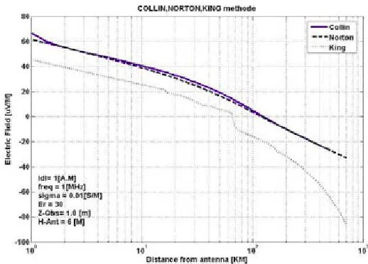
Wait provided a solution for this integral in 1953 which led to figuring out the error function by complex argument [7]. King presented a method to solve the integral in 1969 and 1998 which led to the determination of Fresnel functions [8]. It should be noted that King solved the problem in two cases of flat earth and spherical earth. Of course King Relations are more accurate in high frequencies (f ≥ 1.5 MHz) and high GC (σ > 0.03 S/M). Collin proposed a method in 2004 in which solution of the integral led to computation of error function by complex argument [9]. In this method the earth is also considered flat. Fig. 5 demonstrate these three methods in case of short vertical antenna on earth of characteristics (ε= 30, σ= 0.01 S/M) in f = 1 MHz.
It is observed that Collin’s and Norton’s methods are too close, but there is no sign of earth curve after 100 km in King’s method the earth curve can be observed, but the electric field is less than the previous two methods due to the King’s definition of relation inf = 1–30 MHz. The fracture effect is due to the change of flat earth to spherical earth. In the above mentioned methods the observation point is distant from the antenna, e.g., Collin has used this approximation.
H01(kr)≈
2 πkre
(jk−π
Figure 5. FS of current element in Collin, Norton & King method.
In which the Hankel function holds the first order for great argument approximation, but to determine antenna impedance it is necessary to compute the FS near antenna together with earth effect which is not possible in this method. Here Mie method is used to determine the FS near antenna, which is the base to compute antenna impedance, and Sommerfeld’s integral is not involved.
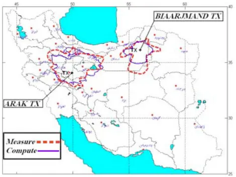
Accurately determining the GC by the use of correctly locating the transmitter’s position has an effective effect on increasing the coverage area of the transmitter. For example, if there are two similar (+) transmitters in area A, one (- - -) near the northern mountains and the other (—) in distance of 150 kM from the previous transmitter, the two transmitters’ difference of coverage area is 4.51% which includes an area of 9025 kM2 of the southern areas. The mountains of the northern area are the reason to the phenomenon; they will cause the field’s contours compress (Fig. 6).
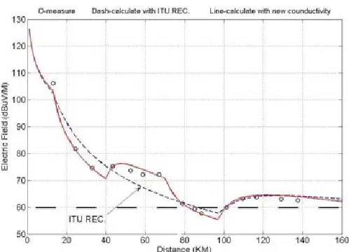
The only reference to GC is the ITU-R P 832-1 [2]. For example, coverage and measurement computation is considered for the transmitters in the desert border. The difference of measurement and computation by the use of the related atlas of the two transmitters in north-eastern (Biaarjomand) & center (Arak) of Iran can be observed in Fig. 7.
Figure 6. Different between coverage of the same transmitter in two points.
Figure 7. Coverage area (Measure and Compute) of Arak & Biaarjmand.
related atlas. The high attenuation due to the two step variation of the GC in mountainous areas is the reason to the congenial converges in the mountainous areas (north) not accuracy in determining GC.
Millington proposed a method to determine FS in inhomogeneous areas [14] which is based on the staircase variation of GC in propagation path. The FS in Y point in the Fig. 8 resulting from the transmitter in theX point is defined as per the below relations.
Figure 8. Propagation path with changing GC in O.
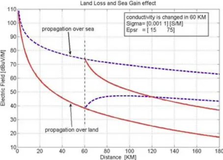
Figure 9. FS over Sea or Land and changing media in 60 KM.
EY = 0.5(EY X+EXY)
In this method, En(dn) is the field from the dn on a surface with ncharacteristics, computable or based on the curves of P 368-7 recommendations [3].
The E1(d1)–E2(d1) value based on σ2 < σ1 or σ2 > σ1 is known as Sea Gain (SG) or Land Loss (LL). In GC atlas one can find paths with quick conductivity and multi step variation, but for sure the variation is constant and through several kilometers. If a GC variation in a distance from 30 kM varies 3 levels, the difference of FS in conductivity variations will be constant and as follows in the staircase (Fig. 10).
Figure 10. FS (dBuV/M) vs. distance for changing the GC (1– 30 mS/M).
Table 2. Earth conductivity in Sirjan. 0.3/6 0.3/6 0.3/6 0.3/6 0.2/4 Dip/Distance
of probes (M)
8.19 6.93 7.37 3.87 2.09 σ(mS/M)
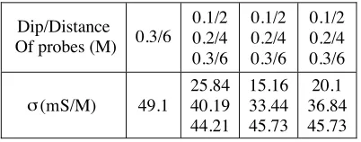
Table 3. Earth conductivity in Maahidasht.
2 / 0.1 4 / 0.2 0.3/6 2 / 0.1 4 / 0.2 0.3/6 2 / 0.1 4 / 0.2 0.3/6 0.3/6 Dip/Distance
Of probes (M)
20.1 36.84 45.73 15.16 33.44 45.73 25.84 40.19 44.21 49.1 (mS/M) σ
2. METHODS TO MEASURE EARTH CONDUCTIVITY
2.1. Measuring Earth Resistivity
The direct measurement of earth resistivity is the first method to measure conductivity [16]. One can mention the following points as the disadvantages of the above method in measuring GC: (A)-Attention is not paid to frequency and its effect. (B)-It cannot analyze parameters like rough earth.
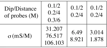
If the aforementioned method is used, there will be a need for modification of relations and making them dependent on frequency. Table 2 shows Sirjaan plateau conductivity with the defined value (σ = 10 mS/M) in 29◦30–34latitude and 55◦43–51longitude, Table 3 shows Maahidasht plateau conductivity with the (σ= 3 mS/M) defined value in 34◦ 8–15 latitude and 46◦ 1–57 longitude and table 4 shows Kermanshah plateau conductivity with (σ= 3 mS/M) defined value in 34◦ 23–28 latitude and 47◦ 0–10 longitude (it should be mentioned that in Table 4, the measurement points head the mountains from plateau which causes decrease in conductivity).
It is realized from tables that GC varies in different depths leading to the point that the method needs modification.
2.2. Measuring Conductivity Based on FS
Table 4. Earth conductivity in Kermanshah.
2 / 0.1
4 / 0.2 2
/ 0.1
4 / 0.2 2
/ 0.1
4 / 0.2 0.3/6 Dip/Distance
of probes (M)
3.014 1.878 6.49 8.921 31.207 76.517 106.103 (mS/M)
σ
(variation of which was not a much easy task). The points around a transmitter in transmitting defined circumstances based on measuring FS, production of an information bank of FS and optimized interpolation are as follows. Then GC is determined based on tables and curves presented [3] from near points assuming the ground around the transmitter as homogenous and determining distant points conductivity based on information of previous points, considering the necessity to use Millington’s algorithm in points where there is unusual variation of electric field. Of course, GC’s staircase variation should be considered too (the above assumption would be problematic regarding the slow variation of GC). The significant points of this method: (1) -Accuracy in transmitter’s important and temporary quantities (transmitter power, antenna gain, antenna and transmitter matching, feeder and antenna system efficiency etc.). (2) -Ground elements existing between the transmitter and the observation point (civil points-rough ground, vegetation cover, etc.) which will be effective in received field.
The information used in this method were applied to transmitter’s related to Tables 2 (two frequency transmitter) and 3 (Figs. 12, 13). The conductivity rate has been drawn regarding distance assuming the homogeneity of the area (which is relatively accurate).
3. THE NEW METHOD TO MEASURE CONDUCTIVITY
In the new method GC is determined based on determining HED antenna impedance near the ground in a way that comparison of antenna impedance in free space and near the ground will provide a criterion to determine GC. To determine GC use is made of an antenna wire which is located near the ground. The antenna impedance variation to antenna impedance in free space is the criterion to determine GC. In the first case the antenna was considered Vertical
Figure 12. GC (mS/M) vs. distance (KM) (ITU ref. 10 mS/M).
Figure 14. Vertical electric dipole on the ground.
Figure 15. Horizontal electric dipole near the ground.
Electric Dipole (VED) which is the common structure used in radio transmitters and the antenna impedance are influenced by two half spaces (the free space & the ground). It can be hypothesized that antenna impedance includes free half space impedance in series with media half space (ground with attenuation) impedance (due to the monopoles in a separate half space) Fig. 14. But as a result of a low impedance obtained from half space 2 in opposition to free space 1 (two impedance series) the GC variation will have a low effect on antenna impedance.
Practically, in radio transmitter to decrease earth effect on antenna impedance and increase radiation power a wire network is set under the antenna so that with increase of conductivity.
3.1. Determining Electric Field by Mie Method
At first, it is reminded to determine the GC with the considered electric characteristics (flat earth along with horizontal antenna, in general solving the not so simple Sommerfeld’s integral) the horizontal antenna is set near the surface of the dielectric sphere with attenuation (εr, σ)
of big radius. If the sphere radius is big enough, the answer to the two problems will be the same. The difference is that solving the problem with the second case is simpler. Mie presented a solution to wave propagation in spherical coordinate in 1908. The electric incident and reflection field (from sphere) resulted from hertz dipole antenna withI current, ∆llength andadorientation in (r0, θ0, ϕ0) point near dielectric sphere with a radius and electric characteristics (εr, σ) in a < r < r0 area are obtained using the relations below (Appendix A).
Ei = ∞
n=1
m=n m=−n
A(4)mnMmn1 (r, θ, φ) +B(4)mnNmn1 (r, θ, φ) (4)
Es = ∞
n=1
m=n m=−n
AsmnMmn4 (r, θ, φ) +BsmnNmn4 (r, θ, φ) (5)
3.2. HED Simulation
The horizontal antenna near the ground was simulated with much smaller horizontal electric currents of to convert the relations above to an applicable mode ∆l≈0.01λwave length. To equalize the figure above with the HED problem, also, the sphere radius was considered a= 5–10λ. The half wave dipole antenna including two monopoles (a quarter of the wave) was located near the sphere (e.g., sphere radius 7λ, each monopole length 0.25λ/7λ= 0.0357rad= 2.05◦ which shows the problem’s proper accuracy in flat earth approximation). Antenna is located inaϕ orientation on z= 0 plate withxaxis centrality or in aϕorientation on y= 0 plate withx axis centrality or any figure with symmetrical state if the antenna distance from the sphere is small enough, d < (λ/500), the antenna can be considered parallel to the surface. The antenna distance (d) from the surface is about 3 mm. After determining electric field with Ei incident and Es scattering
parts, antenna impedance includes inherent impedance (Zi) and the
mutual impedance (Zs). The λ/2 dipole inherent impedance value
is equal to Zi = 7 2 +j46Ω which can be computed and known for
other antenna lengths. The Zs varying the antenna impedance and
Figure 16. HZin vs. Sph. Radius (real(x) imag(o)).
Figure 17. Zin vs. No. of Sum (real(x) image(o)).
In this case antenna impedance is equal to:
Zin = −
1 I2
m λ/4
−λ/4
IantEtant·dl, E t ant=E
i ant+E
s
ant (6)
Zin = 7 2 +j46−
1 I2
m λ/4
−λ/4
IantEants ·dl (7)
In Fig. 16, antenna impedance is drawn in different conductivities for two frequencies based on the dielectric sphere radius (100 constant addition numbers instead of infinity).
Figure 18. impedance based on conduct. (S/M).
and 100 addition number suffices convergence (in extremely specific groundsσ ≤0.0003 S/M radius and addition number should be higher which of course are very rare). In Fig. 18 horizontal antenna impedance is drawn based on GC in different frequencies using Mie method.
A criterion of the (average) area conductivity is obtained measuring antenna impedance in several points (pilot) in the considered area and determining GC based on curves or tables. To ease the use of them, (as recommendation) previous curves are introduced as Table 5.
Table 5. GC vs. HED impedance base on frequency.
HED Antenna Impedance [R + j X]
σ (S/M)
0.5 MHz 0.75 1 1.5
0.001 493 – j 170 630 – j 195 765 – j 218 985 – j 234 0.002 358 – j 231 449 – j 260 545 – j 279 713 – j 299 0.003 274 – j 274 335 – j 304 408 – j 320 541 – j 342 0.004 249 – j 296 300 – j 324 365 – j 339 482 – j 360 0.006 214 – j 328 252 – j 351 303 – j 365 397 – j 384 0.008 193 – j 350 222 – j 370 266 – j 382 345 – j 400 0.010 178 – j 367 204 – j 385 244 – j 398 317 – j 416 0.014 154 – j 393 177 – j 413 215 – j 429 281 – j 449 0.018 137 – j 411 160 – j 435 197 – j 455 261 – j 478 0.022 124 – j 427 148 – j 454 188 – j 477 253 – j 503 0.026 114 – j 440 139 – j470 181 – j496 248 – j 525 0.030 108 – j 450 135 – j483 178 – j 512 246 – j 543
3.3. Measurement Results
The plain and rocky mountains slope of Kermaanshaah area (table 4) were chosen as the practical example. It is reminded that the plain conductivity was several times higher that the mountain slope and the mountain slope measurements are closer to introduced conductivity in recommendation. Measuring was done in 3 frequencies 0.75, 1, 1.5 MHz (each monopole’s length 100, 75, 50 M). To determine the impedance the below antenna measurement set was used. A- Signal Generator RG-4 (Delta Electronics). B- RF BRIDGE 1606B (General Radio Company). C- FS meter FIM-41 (Potomac Instruments Inc.)
Two wires are set in one direction like a dipole. To increase accuracy, antenna average impedance was measured in two measurements perpendicularly (on the ground). Measurements were done after the last spring rain (May 31, 2007) with a gap of seven days. There was no rain during measurement which could change the ground electric characteristic. Fig. 19 shows area’s measurement points.
Table 6. GC in two points base on time.
σ (mS/M) Point s &
Fr eq. (MHz)
Week1 May 31
Week2 Jun 7
Week3 Jun 14
0.75 8.6 8.2 7.8
1 7.2 6.4
A
1.5 5.6 5
0.75 26.3 24.4
1 23.1 20.8
B
1.5 19.2 16.6
7.7 6.2 27.1 24.3 22.4
Figure 19. Measurement points A and B.
4. CONCLUSION
Use of the aforementioned method to determine pilot points GC in the considered area and after that two dimensional interpolations can determine the area conductivity model. In the above method the attenuation influences of crossing rough earth are not predictable.
In digital broadcasting structure, the minimum receivable field and difference of the same channel transmitters’ surface is lower than that of analogue broadcasting to prevent intervention [18]. Besides, it requires higher accuracy of the GC atlas than the present condition to be able to create one frequency channels and to control cover area by the transmitter’s power.
ACKNOWLEDGMENT
Thanks to Mr. AliAsgari deputy of IRIB technical, Mr. Esmaeeli and Mr. Nazari director-general of radio transmitters, Mr. Pahlavani head of research center of radio transmitters for made coordination required for execution of the project.
APPENDIX A.
Solving the Scalar wave equation in spherical coordinates leads to the below equation [19].
Ψgmn(r, θ, φ) = ∞
n=0
n
m=−n
Agmnzn(g)(kr)Pn|m|(cosθ)ejmφ (A1)
If we define (M)T E and (N)T M modes as such: M = ∇ ×(rˆarΨ)
N = 1
k∇ ×(M)
Each one will satisfy the vector wave equation in the spherical coordinates. ∇ × ∇ × M N
+k2
M N = 0 ∇ · M N = 0
In this way (the orthogonal characteristics of the modes to each other) the electric and magnetic fields become
E = ∞
n=1
m=n m=−n
(AmnMmng (r, θ, φ) +BmnNmng (r, θ, φ)) (A2)
H = j η0
∞
n=1
m=n m=−n
In whichM and N are in
Mmn(1),(4)(r, θ, φ) = Mmnr(1),(4)aˆr+M
(1),(4)
mn0 ˆa0+M (1),(4)
mnφ aˆφ
Nmn(1),(4)(r, θ, φ) = Nmnr(1),(4)ˆar+N
(1),(4)
mn0 ˆa0+N (1),(4)
mnφ ˆaφ
Mmnr(1),(4) = 0 Mmnθ(1),(4) = jm
sinθP |m|
n (cosθ)z
(1),(4)
n (kr)e jmφ
Mmnφ(1),(4) = − d dθP
|m|
n (cosθ)z
(1),(4)
n (kr)e jmφ
Nmnr(1),(4) = n(n+ 1) kr P
|m|
n (cosθ)zn(1),(4)(kr)ejmφ
Nmnθ(1),(4) = d dθP
|m| n (cosθ)
1 kr
d dr
rzn(1),(4)(kr)
ejmφ Nmnφ(1),(4) = − jm
sinθP |m| n (cosθ)
1 kr
d dr
rzn(1),(4)(kr)
ejmφ zn1(x) = jn(x), jn(x) =
π 2xJn+12
(x)
zn4(x) = h(2)n (x), h(2)n (x) =
π
2xHn+12(x)
Here jn(x), h2n(x), jn(x), h2n
(x) are spherical Bessel function and related derivatives. Considering the existence of current element (hertz dipole) out of the sphere on (r0, θ0, ϕ0) point with I current and ∆l length and addirection, then
P0=p0ˆad, p0 = I∆l
jω The field inr < r0 is like
E = ∞
n=1
m=n m=−n
A(4)mnMmn1 (r, θ, φ) +Bmn(4)Nmn1 (r, θ, φ) (A3)
H = j η0
∞
n=1
m=n m=−n
A(4)mnMmn1 (r, θ, φ) +Bmn(4)Nmn1 (r, θ, φ) And forr > r0 is like
E = ∞
n=1
m=n m=−n
A(1)mnMmn4 (r, θ, φ) +Bmn(1)Nmn4 (r, θ, φ) (A4)
H = j η0
∞
n=1
m=n m=−n
In which the coefficientsA(1,4), B(1,4) are like A(1)mn,(4) =
−jk3
1p0 4πε
(n− |m|)! (n+|m|)!
2n+ 1
n(n+ 1)ˆad·M (1),(4)
−mn (r0, θ0, φ0)
Bmn(1),(4) =
−jk13p0 4πε
(n− |m|)! (n+|m|)!
2n+ 1 n(n+ 1)ˆad·N
(1),(4)
−mn (r0, θ0, φ0) Which shows application of boundary conditions in r = r0. Now according to the equations, if dielectric sphere ofaradius,εrinsulation
coefficient and σ conductivity are located in center in a way that the source is out of the spherea < r0 for a < r < r0 area of the radiation field is obtained from the below relations
Ei = ∞
n=1
m=n m=−n
A(4)mnMmn1 (r, θ, φ) +Bmn(4)Nmn1 (r, θ, φ) (A5)
Hi = j η0
∞
n=1
m=n m=−n
A(4)mnMmn1 (r, θ, φ) +B(4)mnNmn1 (r, θ, φ)
And the reflected field of the dielectric sphere is obtained according to the relations below.
Es = ∞
n=1
m=n m=−n
AsmnMmn4 (r, θ, φ) +Bmns Nmn4 (r, θ, φ) (A6)
Hs = j η0
∞
n=1
m=n m=−n
AsmnMmn4 (r, θ, φ) +Bmns Nmn4 (r, θ, φ)
Applying the boundary conditions to the sphere surface to make the tangential radiation Ei and reflected fields Es with Et crossing the
Bmns , Asmn coefficients are obtained as below
Asmn = µ2 µ1
ˆ
Jn(ρ1)jn(ρ2)−jn(ρ1) ˆJn(ρ2) h(2)n (ρ1) ˆJn(ρ2)−
µ1 µ2
ˆ
Hn(2)(ρ1)jn(ρ2) A4mn
Bsmn = µ2 µ1 k2 k1 2 ˆ
Jn(ρ1)jn(ρ2)−jn(ρ1) ˆJn(ρ2) h(2)n (ρ1) ˆJn(ρ2)−
µ1 µ2 k2 k1 2 ˆ
Hn(2)(ρ1)jn(ρ2) Bmn4
In which
ρ1 = k1a, k1 =ω√µ0ε0
ρ2 = k2a, k2 =ω√µ0ε2, ε2=ε0
εr2− jσ2 ωε2
In this relationε2 is complex and ˆHn(2)(x),Jˆn(x) is the related Ricotti
Bessel function. ˆ
Jn(x) = d dx
πx 2 Jn+12
(x)
=jn(x) +xjn(x)
ˆ
Hn(2)(x) = d dx
πx 2 H
(2)
n+12(x)
=h(2)n (x) +xhn(2)(x)
REFERENCES
1. International Telecommunication Union (ITU) Recommendations, “Characteristics of AM sound broadcasting reference receivers for planning purposes,” REC. ITU-R BS 703.
2. International Telecommunication Union (ITU) Recommendations, “World atlas of ground conductivities,” REC. ITU-R P 832-1. 3. International Telecommunication Union (ITU) Recommendations,
“Ground-wave propagation curves for frequencies between 10 kHz and 30 MHz,” REC. ITU-R P 368-7.
4. Zenneck, J., “Propagation of plane EM waves along a plane conducting surface,”Ann. Phys. (Leipzig), Vol. 23, 846–866, 1907. 5. Sommerfeld, A. N., “Propagation of waves in wireless telgraphy,”
Ann. Phys. (Leipzig), Vol. 81, 1135–1153, 1926.
6. Norton, K. A., “The propagation of radio waves over the surface of the earth,” Proceedings of the IRE, Vol. 24, 1367–1387, 1936; Vol. 25, 1203–1236, 1937.
7. Wait, J. R., “Radiation from a vertical electric dipole over a stratified ground,”IRE Transaction on Antenna and Propagation, Vol. AP-1, 9–12, 1953; Vol. AP-2, 144–146, 1954.
8. King, R. W. P. and C. Harrison, Jr., “Electromagnetic ground-wave field of vertical antennas for communication at 1 to 30 MHz,” IEEE Trans. on Electromagnetic Compatibility, Vol. 40, No. 4, November 1998.
9. Collin, R. E., “Hertzian dipole radiating over a lossy earth or sea some early and late 20th-century controversies,” IEEE Antenna and Propagation Magazine, Vol. 46, No. 2, Aprill 2004.
10. Arand, B. A., M. Hakkak, K. Forooraghi, and J. R. Mohasel, “Analysis of aperture antennas above lossy half-space,” Progress In Electromagnetics Research, PIER 44, 39–55, 2004.
12. Ruppin, R., “Scattering of electromagnetic radiation by a perfect electromagnetic conductor sphere,” Journal of Electromagnetic Waves and Applications, Vol. 20, No, 12, 1569–1576, 2006. 13. Orizi, H. and S. Hosseinzadeh, “A novel marching algorithm for
radio wave propagation modeling over rough surfaces,” Progress In Electromagnetics Research, PIER 57, 85–100, 2006.
14. Millington, G., “Groundwave propagation over an inhomogeneous smooth earth,”Proceedings of the IEE (UK), Pt. III, 53–64, 1949. 15. Makki, S. V. A. and F. Pahlavani, “Evaluation effect of changing ground conductivity for field strength in MW band,”1st Broadcast Engineering Conference, IRIB Faculty, Tehran, Iran, August 2006. 16. Wenner, F., “A method of measuring earth receptivity,” Report No. Bulletin of Bureau of Standards, Vol. 12, No. 3, Oct. 11, 1915. 17. Xu, X.-B. and Y. F. Huang, “An efficient analysis of vertical dipole antennas above a lossy half-space,” Progress In Electromagnetics Research, PIER 74, 353–377, 2007.
18. Jones, D. S., The Theory of Electromagnetism, Pergamon Press, Oxford, 1964.
19. Li, K. and Y.-L. Lu, “Electromagnetic field from a horizontal electric dipole in the spherical electrically Earth coated with N-layered dielectrics,” Progress In Electromagnetics Research, PIER 54, 221–244, 2005.
20. Mei, J. P. and K. Li, “Electromagnetic field from a horizontal electric dipole on the surface of a high lossy dielectric coated with a uniaxial layer,”Progress In Electromagnetics Research, PIER 73, 71–91, 2007.
21. Abo-Seida, O. M., “Far-field due to a vertical magnetic dipole in sea,”Journal of Electromagnetic Waves and Applications, Vol. 20, No, 6, 707–715, 2006.
22. Liu, C., Q.-Z. Liu, L.-G. Zheng, and W. Yu, “Numeric calculation of input impedance for a giant VLF T-type antenna array,” Progress In Electromagnetics Research, PIER 75, 1–10, 2007. 23. Zhang, H.-Q., W.-Y. Pan, K. Li, and K.-X. Shen,
“Electromag-netic field for a horizontal electric dipole buried inside a dielectric layer coated high lossy half space,” Progress In Electromagnetics Research, PIER 50, 163–186, 2005.