Genus 2 curves with given split Jacobian
Jasper Scholten
[email protected]
November 22, 2018
Abstract
Given 2 Elliptic CurvesE1 andE2, we use some theory of elliptic Kummer surfaces to construct a hyperelliptic curve with Jacobian isogenous to E1 ×E2. We require the 2-torsion of E1 and E2 to be defined over the field we are working over.
1
Introduction
Let E1 and E2 be elliptic curves. The aim of this note is to construct an
explicit genus 2 curve C onE1×E2.
The result of this paper was obtained 15 years ago. At that time I was preparing to write a paper on it, and made a reference to it in another paper [7]. In the proof of lemma 3.1 of [7] a reference to the current paper was made as being in preparation. Since then, results in [7] have been used by other researchers, see [5], [1], [3], [2], and I have been asked about the state of the current paper. This prompted me to finish it.
2
The construction
LetE1 be an elliptic curve given byy12 =f(x1) andE2 an elliptic curve given
by y2
2 = g(x2), with f and g cubic monic polynomials with coefficients in
some field k. Let S be the surface E1×E2/h−1i.
An affine equation for a surface that is birational to S is
with the projection π :E1×E2 →S given by
π(x1, y1, x2, y2)7→(x, y, z) = (x1,
y2
y1
, x2).
Equation 1 occured in work of Kuwata, see for example [4]. It defines an affine part of the associated Kummer surface. See the next section for more on this.
At this point we can jump ahead to the construction of C. After the construction, we will introduce some theory (of elliptic Kummer surfaces) and show why our construction gives the curve we are looking for.
We can consider the equation f(x)y2 −g(z) = 0 as a cubic curve over the rational function field k(y). Call this curve E. Assume that f(x) = x(x−α)(x−β) and g(z) =z(z−γ)(z−δ). The curve E has the following points: (0,0),(0, γ), (0, δ), (α,0), (β,0), (α, γ), (α, δ), (β, γ), (β, δ). By choosing (0,0) as zero point, E becomes an elliptic curve with group law. Denote the group operation by ⊕. We can compute (α, γ)⊕(β, δ). This point over k(y) can be considered as a curve R overk. It is a rational curve on the surfaceS, and its preimageπ−1(R) is the genus 2 curve C onE1×E2
we are looking for.
3
Kummer surfaces
The surface S has singular points at the image of the fixed points of [−1] on E1 ×E2. That is, at the image π(T) for any 2-torsion point T on E1×E2.
There are 16 of those. They are ordinary double points, and blowing them up once resolves the singular point, replacing each point with a P1. This
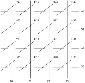
resolution of singularities is called a Kummer surface. Let us call it K and the resulution map ρ : K → S. Figure 1 shows some rational curves on K, and how they intersect:
The curves ρ(Fi) are images π(E1×T) with T a 2-torsion point on E2.
ρ(F0) is the image when T is the zero point of E2.
The curves ρ(Gi) are images π(T ×E2) with T a 2-torsion point on E1.
ρ(G0) is the image when T is the zero point of E1.
The 16 curves Hij are curves created in the blow-ups of singular points
G3
G2
G1
G0
F3 F2
F1 F0
H00 H10 H20 H30
H01 H11 H21 H31
H32 H22
H12 H02
H03 H13 H23 H33
4
Elliptic Surfaces
See [8] for details on this section.
An elliptic surface is a surface X and curve D over a field k and map τ : X → D and a section O : D → X with τ ◦O = IdD such that almost
every fibre τ−1(p) is an elliptic curve with zero O(p). A section is a map ψ :D →X such that the composition τ ◦ψ is the identity map on D. The generic fibre of τ is an elliptic curve over the function field of D. Sections of the elliptic surface are in 1-1 correspondence with points on the generic fibre. We often use the same notation for a point on the generic fibre, its corresponding sectionD→X, and the image of the section, which is a curve on X isomorphic to D.
Some notation: Given two sections F and G, we can add the images as divisors or elements of the N´eron-Severi group. We will denote this sum by F +G. We can also add them using the elliptic curve group law on the generic fibre. This will result in a new section which we denote by F ⊕G.
Singular fibres of an elliptic surface were classified by Kodeira. Once X is non-singular,complete and relatively minimal (one can always find such a model) singular fibres are of type In,II,III, IV, IV∗, III∗, II∗ or In∗.
The N´eron-Severi group N S(X) of a surface X is the group of divisors modulo algebraic equivalence. This group is finitely generated, and there is a pairing on the group, the intersection pairing. For an elliptic surface X, there is a close relationship between N S(X) with the interesection pairing and the Modell-Weil group of its generic fibre with the pairing defined be the N´eron-Tate height. One can define the N´eron-Tate pairing of a point in terms of intersections of the corresponding section with fibre components and the zero-section. For sections (or points on generic fibre) P and Q denote the intersection pairing of P and Qby (P, Q) and the N´eron-Tate height by
hP, Qi. Let χ be the arithmetic genus ofX. Then
hP, Qi = χ+ (P, O) + (Q, O)−(P, Q)−Xcontrv(P, Q), (2)
hP, Pi = 2χ+ 2(P, O)−Xcontrv(P, P).
Here the sums runs over points v ofD such that τ−1(v) is reducible, and the contrv(P, Q) are explicit numbers that depend on the Kodeira type of the
fibre, and which component the sections P and Q intersect.
Any curveP on X that intersects with a fibre once (i.e. (P, τ−1(v)) = 1 for a v onD) is the image of a section.
5
Elliptic Kummer surfaces
A main reference for results in this section is [6].
On a Kummer surface K (or more generally a K3 surface) one can have several different maps to P1 that give it the structure of an elliptic surface.
LetE be a divisor of K such that E is either an elliptic curve, or a reducible curve that is one of the Kodeira types. Then there is a way to give K the structure of an elliptic surface K → P1 such that E is a fibre. The elliptic
surface corresponds to the complete linear system |E|. A few examples of such E are:
• E = 2F0 +H00+ H01 +H02 +H03. This fibre has type I0∗ . This
corresponds to the elliptic surface S → E2/h−1i induced from the
projectionE1×E2 →E2. Other reducible fibres are 2Fi+Hi0+Hi1+
Hi2+Hi3, i≤3, all of typeI0∗.
• Similarly, E = 2G0+H00+H10+H20+H30 of type I0∗, induced from
E1×E2 →E1.
• E = 3F0 + 2H01+ 2H02 + 2H03+G1 +G2 +G3. This has Kodeira
type IV∗. This case corresponds to where consider f(x)y2 −g(z) = 0
as an elliptic curve over k(y). HereE is the reducible fibre over y= 0. There is another reducible fibre of type IV∗ over y = ∞ given by 3G0+ 2H10+ 2H20+ 2H30+F1+F2+F3. The 9 curvesHi,j, 1≤i, j ≤3
are all images of sections (as they intersect the IV∗-fibres once). One can show that they generate a subgroup of the Mordell-Weil group of rank 4, but we won’t need this. In fact, they generate the Mordell-Weil group ifE1 and E2 are not isogenous. IfE1 and E2 are isogenous then
graphs of the isogenies can be used to construct more points, and the Mordell-Weil rank is 4 + rank(Hom(E1, E2)).
6
Computation of intersections and heights
(0, γ), (0, δ), (α,0), (α, γ), (α, δ), (β,0), (β, γ), (β, δ), which by relabeling we assume to correspond to the sectionsH11,H21,H31,H12,H22,H32,H13,H23,
H33 respectively. We choose H11 = (0,0) as the zero for the elliptic curve
group structure. The definition of the elliptic curve group law in terms of lines intersecting the cubic equation (1) in the (x, z)-affine plane over k(y) immediately gives us the following relations:
H13 = H22⊕H32,
H12 = H23⊕H33,
H31 = H22⊕H23,
H21 = H32⊕H33.
LetR denote the curve corresponding to the section H23⊕H32. We will
use the relation between height pairing and intersection pairing to compute the intersection of R with each of the 16 Hij. Note that R is a rational
curve, as it is a section of the elliptic surface over P1. We will find that
(R, Hij) = 2 for exactly 3 pairs (i, j) (namely (i, j) = (0,0),(2,3) and (3,2)),
and (R, Hij) = 0 for all other (i, j). This means that the pullback of R on
E1×E2is unramified outside at most 6 points. The only possible ramification
points are above whereRintersects one of theHij. So the pullback onE1×E2
has genus at most 2. On the singular surfaceSthe curveRhas multiplicity 2 singularities at the points below theHij with (R, Hij) = 2. For now we won’t
study in detail whether the cover ramifies does ramify at these points. In the last section we will obtain an explicit equation of the pullback on E1 ×E2,
and observe that generically it has genus 2.
A IV∗ fibre has 3 components of multiplicity 1. Each section must in-tersect 1 of these. The group structure of the elliptic curve induces a Z/3Z group structure on the 3 components. We use this to determine which re-ducible fibre component intersects the sections we are studying. For a IV∗ fibre, the contrv(P, Q) values are the following:
• contrv(P, Q) = 0 if at least 1 of P and Q intersects the identity
com-ponent.
• contrv(P, Q) = 43 ifP andQintersect the same non-identity component.
• contrv(P, Q) = 23 if P and Q intersect different non-identity
Now we can compute the height pairings and intersection pairings that we need. We start off with using the known intersections between theFi, Gj
and Hij (see figure 1) to compute the height pairings between the 9 sections
Hij,1≤i, j ≤3, using (2). Then we use the bi-linearity of the height pairing
to compute height pairings between other sections. Then we use (2) again to compute the intersection pairings we need.
hHij, Hiji = 4−
4
3 −
4
3 =
4
3 for 2≤i, j ≤3
hH23, H32i = 2−
2 3 − 2 3 = 2 3,
4 = 4
3 + 4 3 + 2 3 + 2
3 = hH23, H23i+hH32, H32i+hH23, H32i+hH32, H23i=
hR, Ri = 4 + 2(R, O), (R, O) = 0,
2 = hR, H23i = 2−(R, H23),
(R, H23) = 0, (R, H32) = 0 is similar
hH23, H33i = 2 + 0 + 0−0−
4 3−
2 3 = 0, 0 = hR, H33i = 2−(R, H33),
(R, H33) = 2, (R, H22) = 2 is similar
2 = hR, H13i = 2−(R, H13),
(R, H13) = 0,
(R, Hij) = 0 for (i, j) = (1,2),(2,1),(3,1) is similar
Note that R does not intersect F0 and G0 because they are fibre
com-ponents with multiplicity >1. And the group law on the component group tells us that it intersects F1 and G1, and it does not intersectF2, G2, F3 and
G3.
Now we have computed (R, Hi,j) for every (i, j) except (i, j) = (0,0).
Since H00 is not a fibre component or section of the elliptic fibration we
chose, we can not use the above technique. However, we can use one of the elliptic fibrations with four I0∗ fibres. Using the intersections computed so far, we can see thatR intersects 3 of theseI0∗ fibres with multiplicity 2, hence it yields a degree 2 cover of Ei/h−1i. Therefore it must also intersect the
7
Explicit Equations
Given the elliptic curve f(x)y2 −g(z) = 0 over k(y) as before, we can use the group law to evaluate
(α, δ)⊕(β, γ) =
(αδ−βγ)(γ−δ)2 (α−β)3y2−(γ−δ)3 ,
(αδ−βγ)(α−β)2y2 (α−β)3y2−(γ−δ)3
To find the Weierstrass points of the genus 2 curve C we are after, we solve for whichythis points passes through (∞,∞), (α, γ) and (β, δ). Our compu-tation of intersection numbers in the previous section ensures that the curve passes through each of these points twice. An easy computation shows that this happens at
y2 = (γ−δ)
3
(α−β)3,
y2 = γ(γ−δ)
2
α(α−β)2,
y2 = δ(γ−δ)
2
β(α−β)2.
So up to a twist, C has equation
Y2 = (α−β)X2−(γ −δ) αX2 −γ βX2−δ
(The ((αγ−−βδ))22 factor can be removed with a straightforward coordinate
trans-formation).
Theorem 1. The curve C defined by equation
(δα−βγ)Y2 = (α−β)X2−(γ−δ) αX2−γ βX2−δ (3)
maps to both elliptic curves E1 and E2.
Proof. Replacing X2 with X maps C to the elliptic curve
(δα−βγ)Y2 = ((α−β)X−(γ −δ)) (αX −γ) (βX −δ) (4) Replacing X with
αδ−βγ (α−β)αβ X+
transforms equation (4) to
α2β2
(δα−βγ)2 Y
2 =X(X−β)(X−α)
which is isomorphic to E1. If we swap α and γ, and we swap β and δ
in equation 3, then the resulting equation defines a curve isomorphic to C
(map X to 1
X and rescale Y). So C also maps toE2.
In the proof of lemma 3.1 of [7] we made use of (a transformation of) equation (3).
References
[1] Daniel J. Bernstein and Tanja Lange. Hyper-and-elliptic-curve cryp-tography. Cryptology ePrint Archive, Report 2014/379, 2014. https: //eprint.iacr.org/2014/379.
[2] Craig Costello. Computing supersingular isogenies on kummer surfaces. Cryptology ePrint Archive, Report 2018/850, 2018. https://eprint. iacr.org/2018/850.
[3] Antoine Joux and Vanessa Vitse. Cover and decomposition index calculus on elliptic curves made practical. application to a seemingly secure curve over Fp6. Cryptology ePrint Archive, Report 2011/020, 2011. https: //eprint.iacr.org/2011/020.
[4] M. Kuwata and T. Shioda. Elliptic parameters and defining equations for elliptic fibrations on a Kummer surface. ArXiv Mathematics e-prints, September 2006. Available at https://arxiv.org/abs/math/0609473.
[5] Fumiyuki Momose and Jinhui Chao. Scholten forms and
ellip-tic/hyperelliptic curves with weak weil restrictions. Cryptology ePrint Archive, Report 2005/277, 2005. https://eprint.iacr.org/2005/277.
[7] Jasper Scholten. Weil Restriction of an Elliptic Curve over a Quadratic
Extension. 2003. Available at http://citeseerx.ist.psu.edu/
viewdoc/download?doi=10.1.1.118.7987&rep=rep1&type=pdf.