Identifying the Future Directions of Australian Excess Stock Returns and Their Determinants Using Binary Models

(1)

Identifying the Future Directions of Australian Excess Stock

Returns and Their Determinants Using Binary Models

Thesis submitted in fulfilment of the requirements for the degree of

Master of Business

College of Business Victoria University

(2)

Abstract

The predictability of excess stock returns has been debated by researchers over time, with many studies proving that stock returns can be predicted to some extent. To enable an effective investment strategy, it is vital for investors to identify the future directions of stock returns and the factors causing directional changes. This study sought to determine whether Australian monthly excess stock return signs are predictable, and identify the key determinants of Australian monthly excess stock return directions. Three different binary models were considered to predict stock directions: discriminant, logistic and probit models. The predictive powers of benchmark static logistic and probit models were also compared with dynamic, autoregressive and dynamic autoregressive models. In order to identify the key determinants, this study considered various economic, international and financial factors, as well as past volatility measures of explanatory variables. It also tested a United States (US) binary recession indicator and Organisation for Economic Co-operation and Development (OECD) composite leading indicator as explanatory variables in the predictive models.

(3)

logistic/probit models showed strong predicting ability, compared to the dynamic, autoregressive and dynamic autoregressive logistic/probit models.

(4)

List of Figures

Figure 1.1: ASX All Ordinaries Index and S&P/ASX 200 Index, January

1990 to December 2014 ... 6 Figure 1.2: Conceptual Framework ... 12 Figure 1.3: Thesis Outline ... 13 Figure 3.1: Monthly Movements of Australian 10-year Bond Yield, 3-month

Bank-accepted Bill Rate and ASX 200 Index, January 1990 to

April 2014 ... 34 Figure 3.2: Monthly Movements of Exchange Rate between AUD/USD and

ASX 200 Index, January 1990 to April 2014 ... 36 Figure 3.3: Monthly Movements of Exchange Rate between AUD/Chinese

Renminbi and ASX 200 Index, January 1990 to April 2014 ... 37 Figure 3.4: Australian Monthly NEs and ASX 200 Index, January 1990 to

April 2014 ... 38 Figure 3.5: Australian Monthly NEs and ASX 200 Index, January 1990 to

April 2014 ... 39 Figure 3.6: Australian Monthly Money Supply (M3) and ASX 200, January

1990 to April 2014 ... 40 Figure 3.7: Australian Monthly Retail Spending and ASX 200 Index, January

1990 to April 2014 ... 41 Figure 3.8: Australian Monthly Private Dwelling Approvals and ASX 200

Index, January 1990 to April 2014 ... 42 Figure 3.9: Australian Monthly Unemployment Rate and ASX 200 Index,

January 1990 to April 2014 ... 43 Figure 3.10: Australian Monthly Index of Commodity Price and ASX 200

Index, January 1990 to April 2014 ... 45 Figure 3.11: World Oil Price Monthly Changes and ASX 200 Index, January

1990 to April 2014 ... 46 Figure 3.12: ASX Monthly PER and ASX 200 Index, January 1990 to April

2014 ... 48 Figure 3.13: ASX Monthly Dividend Yield and ASX 200 Index, January 1990

(8)

Figure 3.14: Monthly MSCI World Index and ASX 200 Index, January 1990 to April 2014 ... 51 Figure 3.15: Monthly Movements of S&P 500 and ASX 200 Indices, January

1990 to April 2014 ... 53 Figure 3.16: Monthly Movements of US 10-year Bond Yield, US 90-day Bill

Rate and ASX 200 Index, January 1990 to April 2014 ... 54 Figure 3.17: Monthly Movements of OECD Leading Indicator and ASX 200

Index, January 1990 to April 2014 ... 56 Figure 3.18: Binary Recession Indicator and ASX 200 Monthly Movements,

(9)

List of Tables

Table 4.1: Explanatory Variables of Binary Models ... 71

Table 5.1: Estimated Discriminant Models, January 1990 to May 2012 ... 75

Table 5.2: Correlation Matrix ... 78

Table 5.3: Statistically Significant Explanatory Variables in Discriminant Analysis ... 78

Table 5.4: Most Important and Strong Predictors Based on Discriminant Analysis ... 80

Table 5.5: Classification Results of Discriminant Models ... 82

Table 5.6: Estimated Logistic Models, January 1990 to May 2012 ... 85

Table 5.7: Estimated Probit Models, January 1990 to May 2012 ... 87

Table 5.8: Statistical Significance of Explanatory Variables in Probit and Logistic Analysis ... 90

Table 5.9: Classification Results of Logistic Models ... 91

Table 5.10: Best Discriminant Models ... 94

(10)

List of Abbreviations

ANOVA Analysis of Variance APT Arbitrage Pricing Theory

ASX Australian Security Exchange Limited AUD Australian Dollar

CAPM Capital Asset Pricing Model CC2 _{Squared Canonical Correlation} CPI Consumer Price Index

GDP Gross Domestic Product LR Likelihood Ratio

MAD Mean Absolute Deviation

NBER National Bureau of Economic Research

NE Net Export

OECD Organisation for Economic Co-operation and Development OLS Ordinary Least Squares

PER Price/Earnings Ratio S&P Standard and Poor SD Standard Deviation

U2 _{Squared Return}

US United States

(11)

Master by Research Declaration

‘I, Chinthana Sanjeewa Bandara Hatangala, declare that the Master by Research thesis entitled Identifying the Future Directions of Australian Excess

Stock Returns and Their Determinants Using Binary Models is no more than

60,000 words in length, including quotations and excluding tables, figures, appendices, bibliographies, references and footnotes. This thesis contains no material that has been submitted previously, in whole or in part, for the award of any other academic degree or diploma. Except where otherwise indicated, this thesis is my own work.’

(12)

Acknowledgements

I would like to take this opportunity to express my gratitude to Associate Professor Nada Kulendran, College of Business, Victoria University. I was fortunate to have him as my principle supervisor, and my thesis would have not been possible without his support. I am thankful for his aspiring guidance, expert knowledge, professional supervision and friendly advice throughout my studies.

I also wish to express my gratitude to my associate supervisor, Dr Ranjith Ihalanayaka, College of Business, Victoria University, who was abundantly helpful throughout my studies. I offer my sincere appreciation for his invaluable support, expert advice and comments upon completion of my thesis.

I would also like to thank Ms Tina Jego, Senior Officer, Graduate Research Centre, Victoria University, for her professionalism, kindness and administrative support provided to me from day one.

I can never thank enough my father Dayasena, mother Kamala and brother Pubudu, who have given me continued support and encouragement throughout my studies.

(13)

Publications Associated with Thesis

Hatangala C & Kulendran N 2014, ‘Identifying the future directions of the Australian stock returns and their determinants using binary models’, paper presented at the 31st Annual Pan-Pacific Conference, 2–5 June, Sakai City,

(14)

Chapter 1: Introduction

1.1 Research Background

Investor interest in stock market investments remains consistently high, despite the uncertainty of returns. This is largely due to the extra returns that can be earned from the stock market, in comparison to safer investments, such as government securities and bank deposits. The extra returns of stock investments are the expected return of stock investments that surpass the risk-free return (the return of government securities)—known as ‘excess stock returns’. Generally, investors allocate a significant proportion of their funds to the stock market, and the proportion of investment varies depending on the future expectations of excess stock returns. Investors allocate a higher proportion of funds to stock investments when the expected excess stock returns are high. In contrast, funds are transferred to risk-free alternatives when the expected excess stock returns are low.

(15)

Potter (2001), in stock market terminology, bull (bear) markets correspond to periods of generally increasing (decreasing) market price.

In recent years, stock prices around the world have been very sensitive not only to corporate announcements, such as the release of financial results, dividend announcements and changes to boards of directors but also to macroeconomic changes. Since the Global Financial Crisis that began in mid-2007 in the United States (US), stock investors have become more alert of changes in economic conditions than ever before. Today’s stock prices not only reflect the expected financial performance of companies, but also quickly adjust to changes that occur in macroeconomic and international factors.

Various methods and econometric models have been developed to forecast the value and directional changes of stock returns. Based on this, two main types of forecasting models are identified in the literature: classification models and level estimation models. Classification models are used to predict the directional changes of stock returns, while level estimation models are used to predict the values of stock returns. Several studies have identified classification models as the better of these two types of model in terms of forecasting accuracy. Leung et al. (2000) demonstrated that the group of classification models is superior to the group of level estimation models in terms of forecasting stock market movements because classification models are able to generate higher trading profits than are level estimation models.

(16)

number of studies have demonstrated that binary models have better predictive power than level estimation models. For example, Leung et al. (2000), Nyberg (2008) and Hong and Chung (2003) used various multivariate binary classification models to predict stock returns, including linear discriminant analysis, logit, probit and probabilistic neural network models. Their empirical results suggested that the binary classification models outperformed the level estimation models, and that binary models are strong in predicting the direction of stock market movements and maximising returns from investment trading.

(17)

Researchers have identified significant relationships between economic conditions and excess stock returns in many empirical studies. For example, Chauvet and Potter (1998) found a time-varying relationship between stock return and risk in regard to business cycle turning points. Fama and French (1989) and Whitelaw (1994) also found a significant dependency relationship in the conditional distribution of stock returns and business conditions. These studies have revealed that, when economic conditions are good, stock markets follow a bull-run, in which excess stock returns increase. In contrast, when economic conditions are bad, the market follows a bear-run, in which excess stock returns decrease. In another study, Chauvet and Potter (2000) established that a bear market generally begins a couple of months before an economic contraction, and ends before the trough of recession. Nyberg (2008) established that binary dynamic regression models can be successfully used to predict US monthly excess stock returns. His study also showed that models that used the binary recession indicator as an explanatory variable outperformed models that used only the financial variables.

(18)

logistic and probit models, this study used dynamic, autoregressive and dynamic autoregressive models for sign forecasting. Autoregressive models and dynamic autoregressive models (new dynamic models) were proposed by Kauppi and Saikkonen (2008) to predict US recession periods.

This study tested various economic, financial and international variables as explanatory variables of predictive models to identify the key determinants of Australian monthly excess stock return directions. This study also tested how different past volatility measures of selected predictor variables can be used in binary models to forecast stock returns. US binary recession indicators were first used by Nyberg (2008) to predict US stock market directions, and were tested in the current study as an explanatory variable to forecast Australian stock market directions. Further, the Organisation for Economic Co-operation and Development (OECD) index for Australia—a composite leading indicator intended to forecast Australian future economic activity—was tested as an explanatory variable to predict excess stock return signs.

1.2 Australian Stock Market and S&P/ASX 200 Index

(19)

consists of market capitalisation of the top 500 companies, and still runs parallel to the S&P/ASX 200. However, the S&P/ASX 200 is considered the major index to represent Australian stock exchange movements. This study sought to predict the monthly movements of the S&P/ASX 200 index. Figure 1.1 illustrates the perfectly positive relationship between the ASX All Ordinaries and S&P/ASX 200 index.

Figure 1.1: ASX All Ordinaries Index and S&P/ASX 200 Index, January 1990 to December 2014

Source: DX Database & www.rba.gov.au/statistic.

1.3 Aims of the Study

The main aim of this study was to predict the directional change in Australian monthly excess stock returns using binary models, and identify the key contributory factors that determine the monthly directions of excess stock returns in Australia. The specific aims of the study were as follows:

(20)

1. To assess the forecasting accuracy of three binary models— discriminant, logistic and probit models—for predicting Australian monthly excess stock return signs.

2. To measure the success of using developed binary models—such as dynamic logit/probit, autoregressive and dynamic autoregressive models—in predicting Australian excess stock returns, in comparison to benchmark static models.

3. To identify the major economic and financial factors that are significant in predicting Australian stock return signs.

4. To determine how international stock markets, such as the S&P 500 index and MSCI world index, affect the monthly direction of Australian stock returns.

5. To evaluate the effect of US economic indicators on the monthly direction of Australian stock returns.

6. To measure the effect of leading economic indicators—such as the OECD indicator and US recession indicator (dates defined by the US National Bureau of Economic Research)—on Australian stock return directions.

7. To examine the use of different past volatility measures of predictor variables—such as the mean absolute deviation (MAD), standard deviation (SD) and squared return (U2_{)—in predicting directional changes} in Australian stock returns.

(21)

1.4.1 Research Question 1

Are the directions of monthly Australian excess stock returns predictable using discriminant, logistic and probit models?

Do the developed dynamics probit/logit, autoregressive and dynamic autoregressive models offer better predicting results than benchmark static models in predicting Australian excess stock return signs?

What are the key economic and financial factors that drive excess stock return directions?

Are global stock market movements significant in predicting Australian excess stock return signs?

Which US economic indicators are significant in predicting Australian excess stock return signs?

(22)

Which volatility measures of predictor variables can be used to forecast excess stock return directions using binary regression models?

1.5 Contribution to Knowledge (Academic Contribution)

Classification models have been widely used by scholars around the world to predict the directions of growth cycles, such as business, stock return and tourism growth cycles. A number of studies have shown that binary classification models compare favourably with other predictive models—such as level estimation models—in predicting growth cycles. Although some studies have used binary models to forecast the directions of international indices, such as the S&P 500, only a few studies have used binary models to predict the future directions of Australian excess stock returns.

This study focused on assessing the ability of three major binary models— discriminant, logistic and probit models—to predict the monthly directions of Australian excess stock returns. To the best of the researcher’s knowledge, this is the first study to use dynamic binary models to predict Australian stock market directions. This study sought to assess how new dynamic logistic and probit models introduced by Kauppi and Saikkonen (2008) can be used to predict Australian monthly excess stock return signs.

(23)

S&P500, MSCI and foreign exchange rate—are significant in predicting excess stock return signs. It tested three different volatility measures (MAD, SD and U2₎ of selected predictor variables to assess their predictive power for Australian excess stock return signs. This type of analysis is important to study how predictive power changes when considering the volatility of predictor variables, and to assess the effectiveness of different volatility measures to predict ASX returns.

In addition, this study employed business cycle leading indicators—such as the OECD index and US binary recession indicators—as explanatory variables to evaluate their predictive ability for Australian excess stock return directions. To the best of the researcher’s knowledge, no previous study has used business cycle leading indicators to predict Australian excess stock return directions.

1.6 Statement of Significance (Practical Contribution)

(24)

study makes an important contribution to stakeholders—such as investors, equity analysts, fund managers, researchers and investment policy makers— who are interested in the future directions of Australian excess stock returns and the key factors driving those directions.

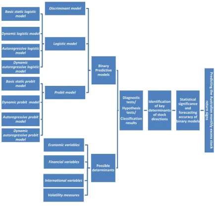
1.7 Conceptual Framework

(25)

Figure 1.2: Conceptual Framework

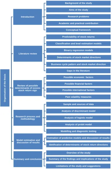
1.8 Thesis Outline

This section describes the outline of the thesis, as shown in Figure 1.3.

Predicti n g th e A u str al ia n month ly exc ess stoc k retu rn signs Statistical significance and forecasting accuracy of binary models Identification of key determinants of stock directions Diagnostic tests/ Hypothesis tests/ Classification results Binary Predictive models Discriminant model Logistic model Basic static logistic

model Dynamic logistic model Autoregressive logistic model Dynamic autoregressive logistic model Probit model Basic static probit

model Dynamic probit model

(26)

Figure 1.3: Thesis Outline

O

rganisatio

n

of

th

e

th

esis

Introduction

Background of the study

Aims of the study

Research problems

Academic and practical contribution

Conceptual framework

Literature review

Predictability of stock returns

Classification and level estimation models

Binarry regression models

Business cycle pattern and stock market direction Determinants of stock market directions

Gaps in the literature

Review of possible determinants of excess

stock return sign

Possible economic factors

Possible financial factors

Past volatility measures Possible international factors

Research process and methodology

Sample and sources of data

Analysis of discriminant model

Analysis of logistic model

Analysis of probit model

Modelling and diagnostic testing

Model estimation and discussion of results

Estmation of predictive models and discussion of results

Idetification of determinants of stock return directions

Summary and conclusion

Overview of the study

(27)

Chapter 1: Introduction

The first chapter introduces the research. It explains the study background, aims, research problems, and academic and practical contributions. It also discusses the thesis’s conceptual framework and structure.

Chapter 2: Literature Review

The literature review chapter presents a comprehensive review of past studies related to forecasting the directions of stock returns and the key determinants of stock return future directions. This chapter comprises sections that discuss previous studies testing the predictability of stock returns, a comparison of classification models and level estimation models for stock return predictions, the theoretical background for identifying the determinants of stock return directions, the relationship between business cycle patterns and stock market directions, economic international and fundamental financial factors for predicting stock returns, and the use of leading economic indicators to forecast stock directions. Finally, this chapter discusses the gaps in the relevant literature.

Chapter 3:Review of Possible Determinants of Excess Stock Return Signs

(28)

Chapter 4: Research Process and Methodology

Chapter 4 discusses the research process and methodology used to predict Australian monthly excess stock return signs and identify the key determinants. Further, it discusses the sample and sources of data collected for the study. It explains the three binary models employed—discriminant, logistic and probit models—and the developed dynamic logistic/probit models. It also discusses the modelling and diagnostic tests used for the discriminant, logistic and probit models.

Chapter 5: Model Estimation and Discussion of Results

Chapter 5 presents the results of the estimated binary predictive models. It identifies the best binary models for predicting Australian monthly stock returns, based on goodness-of-fit measures and forecasting accuracy (hit ratio). It also identifies the determinants of the monthly directions of stock returns.

Chapter 6: Summary and Conclusion

(29)

Chapter 2: Literature Review

2.1 Introduction

This chapter reviews the literature related to predicting stock returns and their determinants, comprising six sections. The first section discusses previous studies that tested the predictability of stock returns. The second section explains previous studies’ use of classification models and level estimation models to forecast stock returns. The third section discusses previous studies’ use of binary models as level estimation models to predict stock signs. The fourth section discusses the literature that studied the determinants of excess stock returns and the theoretical background of identifying determinants. It also reviews the existing literature related to the possible determinants of stock market returns, including economic factors, international factors, the volatility of past returns and fundamental financial factors. The final section identifies the gaps in the literature and summarises the chapter.

2.2 Is the Direction of Stock Return Changes Predictable?

(30)

The efficient market hypothesis implies that stock price movements are based on the random walk hypothesis and are unpredictable. However, theories and studies supported the efficient market hypothesis (that is stock returns are unpredictable) has been revised by new empirical findings in recent years. New empirical findings have revealed that market directions are predictable and that past prices, past volatility and other independent determinants can be used to forecast future stock price movements, to some extent. For example, Breen et al. (1989) developed a forecasting model based on the negative relationship between stock index returns and treasury bill interest rates, and assessed the forecasting ability of stock returns. This study used two market timing tests—the Cumby-Modest and Henriksson-Merton tests—to demonstrate that treasury bill returns can forecast changes in the distribution of stock index excess returns.

(31)

views of returns are independent overtime. Thus, based on this review of past studies, a number of outcomes have demonstrated that stock returns are predictable, to some extent.

2.3 Level Estimation and Classification Models for Stock Return

Predictions

In reviewing previous studies that addressed the predictability of excess stock returns, two main branches of predictive models were identified. Some research used level estimation models that forecast the value of excess stock returns, while others used classification models that predict the directions of stock indices. However, in recent years, there has been a growing focus on predicting the directions of share returns or market indices, rather than predicting exact values.

(32)

forecast the stock market’s level—both in terms of the accuracy of predicting the directions of stock market movement, and maximising returns from investment trading.

In another study, Enke and Thawornwong (2005) examined the effectiveness of the neural network level estimation and neural network classification models. They concluded that the trading strategies guided by neural network classification models generate higher profits under the same risk exposure than the buy-and-hold strategy, as well as the level estimation forecast of neural network. In addition, based on conventional forecast error magnitude criteria, Leitch and Tanner (1991) found that predicting the direction of change in profitability is the best criterion for investment decisions, rather than forecasting profit based on values.

2.4 Using Binary Regression Models as Classification Models

for Sign Predictions

(33)

empirical results suggested that the binary classification models outperformed the level estimation models, and that the binary models were strong in predicting the direction of the stock market movement and maximising returns from investment trading.

Hong and Chung (2003) also examined the out-of-sample profitability of a class of binary logistic models for directional forecasts of excess returns, and found that trading rules based on logistic forecast models could earn significantly higher risk-adjusted returns than trades based on the buy-and-hold strategy. In another study, Nyberg (2008) studied the predictive power of dynamic binary probit models developed over a period of time, and found that the number of correct signs (hit ratio) of US monthly returns and investment returns were higher when using dynamic probit models, as opposed to their level estimation counterparts.

2.5 Determinants of Excess Stock Return Directions

(34)

2.5.1 Theoretical Background to Identify Determinants of Excess Stock Return Directions

The CAPM, APT and dividend discount model can be used to explain the relationship between economic activity and stock market direction. These are further reviewed in the following sections.

CAPM

The CAPM developed by Sharpe (1964), Lintner (1965) and Mossin (1966) explains the relationship between macroeconomic forces and share returns. The CAPM explains the price of securities built on the relationship between the expected return of the stock (E[r]) and market risk. Market risk arises due to changes in macroeconomic variables, and these changes affect stock returns as per the model. The CAPM model explains stocks returns as E(r) = rf + β (rm − rf), where rf is the risk-free interest rate, (rm − rf) is the market risk premium and β (beta) is the sensitivity of stock returns to market risk. The market risk premium changes due to changes in macroeconomic variables, and these changes then affect stock returns and market price.

APT

(35)

model) is more general than the CAPM when understanding the relationship between stock returns and market forces.

Dividend Discount Model

The dividend discount model developed by Gordon and Shapiro (1956) can also be used to express the relationship between economic forces and stock prices. The dividend discount model is defined with the formula:

n t

t k

D ice

Stock

) 1 ( Pr

1 

 





where Dt is the expected dividend stream and k is the required rate of return. According to this model, the systematic economic forces that influence corporate earnings (Dt/cash flows) and required rate of return (risk-free rate and market risk premium) determine the share price and excess stock returns.

2.5.2 Past Volatility of Stock Returns to Forecast Future Directions

(36)

relationship between asset return volatility and asset return sign forecasts, and found that sign probability forecasts are most sensitive to changes in volatility at an intermediate level (two to three months). In another study, Breen et al. (1989) demonstrated that a positive expected excess return—or the probability of an up market—is a function of conditional variance of past returns.

2.5.3 Business Cycle Pattern and Market Directions

A number of previous studies have identified the condition of the economy as the most critical factor for predicting excess stock returns. Fama and French (1989) found a clear business cycle pattern for expected returns on common stocks. They stressed that expected returns are low near peaks and high near troughs of the business cycle. Further, they identified that expected returns contain a risk premium that is related to longer-term aspects of the business condition, and revealed that changes to the risk premium are stronger for stocks as business conditions change.

(37)

volatility, investors might move back and switch from stock to bond, thereby driving changes in expected returns and the direction of the relationship, depending on the stage of the economy.

Economic and International Factors to Forecast Future Stock Directions

Many scholars have discussed how changes in various macroeconomic factors affect excess stock returns. Previous studies have tested various macroeconomic variables as predictive variables to forecast stock returns. Fama and Schwert (1977) estimated the extent to which stock returns are predictable using the expected and unexpected components of the inflation rate during the period 1953 to 1971. They used the Consumer Price Index (CPI) and returns on an equally weighted portfolio and value-weighted portfolio of New York Stock Exchange stocks. They found that common stock returns are negatively related to the expected component of inflation and are probably related to the unexpected component of inflation. In another study, Breen et al. (1989) constructed a forecasting model based on the negative correlation between stock index returns and treasury bill interest rates, and concluded that treasury bill returns can successfully forecast changes in the distribution of stock index excess returns.

(38)

and high-grade bonds). Further, they concluded that stock returns are exposed to systematic economic news and priced in accordance with their exposures. Chen (1991) showed that state variables—such as the lagged production growth rate, term premium and short-term interest rate—are reliable indicators of recent and future economic growth. Chen further revealed that excess market returns are negatively correlated with recent economic growth and positively correlated with expected future economic growth.

In another study, Pesaran and Timmermann (1995) examined the predictive power of various economic factors over the monthly stock return change, such as the treasury bill rate, treasury bond rate, industrial output, inflation and money supply. They examined the period between 1954 and 1992, and concluded that predictability seemed quite low during relatively calm markets, and increased when the market was more volatile. A study by Whitelaw (1994) stated that the economic variables such as bond yield spread, interest spread between commercial papers and one year treasury yield, and dividend yield combinedly provides reasonable evidence of predictability in both returns and their volatility. Based on US excess stock returns forecast, Campbell and Thompson (2008) demonstrated that macroeconomic variables—such as short- and long-term interest rates, level of consumption and stock market valuation ratios—provide a better out-of-sample prediction than the historical average return forecast.

(39)

long term. The study suggested that, in the long term, Australian stock market returns are influenced by systematic risk factors, such as interest rates, corporate profitability, industrial production and (to a lesser extent) global market movements. In the short term, it is adjusted each quarter by its own performance, interest rates and global stock movements of the previous quarter.

Kearney and Daly (1998) examined how the conditional volatility of Australian stock market returns is related to the conditional volatility of financial and business cycle variables. They estimated the conditional volatility of stock market returns using the generalised least squares model, examining monthly data over the period of 1972 to January 1994. They found a strong association between the conditional volatility of money supply and conditional volatility of Australian stock market returns. Further, they revealed that the conditional volatilities of inflation and interest rates are directly associated with stock market volatility. They also found that current account deficits, industrial production and money supply are indirectly associated with stock market volatility. However, they found no evidence of a statistically significant relationship between foreign exchange markets and the Australian stock market.

(40)

Shamsuddin and Kim (2003) examined the integration of the Australian stock market with two leading trading partners—the US and Japan—prior to and following the Asian financial crisis. They found that there was a long-term relationship between the Australian, US and Japanese markets prior to the crisis; however, the US influence on the Australian market diminished in the post-crisis period even though US influence on Japan remained at a modest level. They also found that the Australian market became more independent with country’s own factors after the financial crisis.

Di Lorio and Faff (2000) examined the foreign currency exposure of Australian equities market major sectors using AUD/USD factor return in an augmented market model. Their results were quite mixed, with nine industries showing significant exchange rate exposure—oil and gas, solid fuels, alcohol and tobacco, chemicals, engineering and retail, food and households goods, property trust and building materials.

Leading Economic Indicators to Forecast Future Stock Directions

(41)

inbound-tourism growth cycle. They stressed the importance of using separate composite leading indicators for each source market in future research.

The recession dates defined by National Bureau of Economic Research (NBER) in the US is one of the leading indicators used to identify US business cycle patterns. Nyberg (2008) studied the ability of dynamic probit models to predict the direction of monthly US excess stock returns signs. Nyberg introduced a binary recession indicator that was estimated based on NBER recession dates as an explanatory variable in the predictive model. This was the first time this approach had been used to forecast stock return signs. The study employed and extended new dynamic probit models proposed by Kauppi and Saikkonen (2008). The empirical results showed that, when these models used the six-month recession forecast as an explanatory variable, they outperformed other predictive models that used only financial variables as explanatory variables.

2.5.4 Fundamental Financial Variables to Forecast Future Stock Directions

(42)

growth, whereby economic growth is positively correlated to excess stock returns. Cochrane (1999) found that the expected return on individual securities and the market as a whole varies slowly over time; thus, the market expectation of returns can be tracked by watching the price/dividend ratio, PER or book/market ratio. Pesaran and Timmermann (1995) examined the predictive power of various economic factors—including earnings per share and dividend yield over monthly stock return change—and concluded that variables have a predictive power over stock returns. In addition, Whitelaw (1994) stated that dividend yield can be used to predict variation in both returns and their volatility. Kazi (2009) suggested that, in the long term, Australian stock market returns are influenced by only a few factors, which include dividend yield.

2.6 Gaps in the Literature and Chapter Summary

(43)

Business cycle patterns in regard to stock market directions have been considered in previous studies, with various macroeconomic, financial and international factors identified as determinants of stock directions. Although some researchers have used leading indicators as predictor variables in binary models to forecast business cycles and global stock market directions, there has been no such study related to the Australian stock market. Thus, the current study used an OECD indicator to predict Australian stock directions. The Australian OECD indicator is a designed composite leading indicator for Australia to measure the country’s economic activity and identify early signals of turning points in economic activity. The study by Nyberg (2008) used a US binary recession indicator (based on recession dates defined by the NBER) for the first time to forecast US stock directions, and concluded that recession indicators are a useful predictor variable. Considering the strong association between the US economy and Australian stock market, the current study also sought to test a US recession indicator for the first time to predict Australian stock directions.

(44)

Chapter 3: Review of Possible Determinants of

Australian Excess Stock Return Signs

3.1 Introduction

The latter part of the previous chapter presented a review of the various determinants of stock market directions, and how these determinants have evolved over time. This chapter discusses the possible determinants that were examined in this study to predict Australian monthly excess stock return signs.

3.2 Selecting Possible Determinants of Australian Monthly

Stock Directions

(45)

3.2.1 Interest Rates

The interest rates of an economy play a critical role in investment strategy and asset allocation decisions. Interest rates are the key indicator of the rate of return on debt investments, including government securities. Given their role in investment decisions, it is important to identify what relationship exists between interest rates and excess stock returns.

Excess return (rt) is the investment return of equity investments that exceeds the risk-free interest rate. The risk-free interest rate (rf) is a fragment of the formula used to calculate excess stock returns (rt = Ln (Pt/Pt−1) − rf) and, when the risk-free interest rate is low, the excess return is high, and vice versa. In addition, the CAPM used to explain the required rate of return (RRR = rf + β [rm − rf]) can be used to identify the relationship between interest rates and investment decision making. When rf is high, there is a higher required rate of return for investments compared to the expected returns of the investment, and vice versa. If the expected return does not meet or exceed the required return, the investment should not proceed.

From another perspective, lower interest rates improve the future earnings and cash flows of companies. Especially for high-geared companies, the cost of borrowing will be low in low-interest-rate scenarios, which improves the company’s profits. Also, when the future interest rate outlook is positive or remains at lower levels, consumer spending improves and business confidence is boosted, which helps improve stock prices.

(46)

attractiveness of debt security investments, such as bonds (market price increase), which moves investors to the equity market to earn more returns. Investments by foreign investors also affect the interest rate in Australia—low interest rates in Australia compared to the international market increase foreign investor confidence in Australian businesses.

The inverse relationship between interest rates and stock returns has been explained in several previous studies. Alam and Uddin (2009) studied the relationship between interest rates and stock returns in 15 stock markets, including the Australian stock market, based on time series and panel regression. They concluded that interest rates have a strong negative relationship with all the stock markets they reviewed. Campbell (1987), Whitelaw (1994), Kazi (2009) and Erdugan (2012) all found that interest rates can be used successfully to forecast stock returns, with both short- and long-term interest rates and long-term structures considered successful predictive variables of stock return directions.

To measure the effect of interest rates on the monthly directional changes of Australian excess returns, this study considered different measures of interest rates:

 short-term interest rates (three-month bank-accepted bill rate for

Australia)

 long-term interest rate (10-year bond yield for Australia)

(47)

 term spread (difference between a 10-year bond yield and three-month

bank-accepted bill rate).

Figure 3.1 illustrates the relationship between the ASX 200 index and Australian short- and long-term interest rates. This illustration indicates that an inverse relationship existed between interest rates and the ASX 200 index from 1990 to 2014.

Figure 3.1: Monthly Movements of Australian 10-year Bond Yield, 3-month Bank-accepted Bill Rate and ASX 200 Index, January 1990 to April 2014

Data source: DX Database & www.rba.gov.au/statistic.

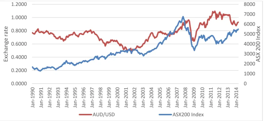
3.2.2 Foreign Exchange Rate

The exchange rate between the AUD and other currencies is determined by the demand for and supply of the AUD as a result of international activities with foreign countries. The AUD is one of the critical factors influencing the earnings of domestic companies, depending on their exposure to international trade. Companies who do not engage in much international trade and are mainly

0 1000 2000 3000 4000 5000 6000 7000 8000 0.00 2.00 4.00 6.00 8.00 10.00 12.00 14.00 16.00 18.00 20.00 Jan -1990 Jan -1991 Jan -1992 Jan -1993 Jan -1994 Jan -1995 Jan -1996 Jan -1997 Jan -1998 Jan -1999 Jan -2000 Jan -2001 Jan -2002 Jan -2003 Jan -2004 Jan -2005 Jan -2006 Jan -2007 Jan -2008 Jan -2009 Jan -2010 Jan -2011 Jan -2012 Jan -2013 Jan -2014 AS X 20 0 Ind ex Interes t rate(%)

(48)

focused on the Australian market benefit from depreciation of the AUD against other currencies. Depreciation of the AUD favourably affects these companies because foreign goods and services are relatively expensive for domestic buyers. However, when the AUD appreciates against foreign currencies, imported products are cheaper for domestic buyers, which adversely affects domestic companies who are less involved in international trade.

Changes in the foreign exchange rate also play an important role in the level of foreign investments in the local share market. In Australia, a significant proportion of the stock market is owned by offshore investors, and their reaction is an important factor determining the direction of Australian stock returns. The Australian share market is not attractive to international investors when the AUD is trading at high levels compared to the domestic currencies of foreign investors. In contrast, when the AUD is trading at low levels, international investors’ interest in buying Australian shares increases, and stocks become more attractive to foreign investors.

(49)

(positive or negative exposure) for different industry categories in the stock market.

In the current study, the exchange rate between the AUD and USD (AUD/USD) and the AUD and Chinese renminbi (AUD/REN) were considered predictive variables of binary models. The US exchange rate is an international standard unit of currency, and the also US is the second-largest trading partner of Australia an over a period of time. The Chinese renminbi exchange rate was also considered a predictor variable, given China’s involvement with the Australian economy, with China being Australia’s largest trading partner in terms of both imports and exports. Figures 3.2 and 3.3 demonstrate the relationship between the ASX 200 index and the two exchange rates. Both the AUD and Chinese renminbi display a negative relationship with the ASX 200 over the period considered, but a positive relationship during recession time from 2007 to 2009.

Figure 3.2: Monthly Movements of Exchange Rate between AUD/USD and ASX 200 Index, January 1990 to April 2014

0 1000 2000 3000 4000 5000 6000 7000 8000 0.0000 0.2000 0.4000 0.6000 0.8000 1.0000 1.2000 Jan -1990 Jan -1991 Jan -1992 Jan -1993 Jan -1994 Jan -1995 Jan -1996 Jan -1997 Jan -1998 Jan -1999 Jan -2000 Jan -2001 Jan -2002 Jan -2003 Jan -2004 Jan -2005 Jan -2006 Jan -2007 Jan -2008 Jan -2009 Jan -2010 Jan -2011 Jan -2012 Jan -2013 Jan -2014 AS X 20 0 Ind ex Exchan ge rate

(50)

Figure 3.3: Monthly Movements of Exchange Rate between AUD/Chinese Renminbi and ASX 200 Index, January 1990 to April 2014

3.2.3 Export and Imports

Australia is one of the leading suppliers of natural resources to the world market, and is ranked in the top 20 economies in terms of global trade. From 2014 to 2015, the value of total exports of goods and services was recorded as AUD$318.7bn, which accounted for over two per cent of the country’s gross domestic product (GDP), with China, Japan and the US the three major trading partners. The net export (NE) is the difference between a country’s export and import of goods and services. Positive NE (trade surplus) is considered favourable for a country’s economic growth. Balassa (1986), Ram (1985) and Tyler (1981) highlighted the positive relationship between export growth and level of economic development. The current study tested the monthly exports, imports and NEs (exports − imports) as predictive variables of ASX 200 monthly

0 1000 2000 3000 4000 5000 6000 7000 8000 0.0000 1.0000 2.0000 3.0000 4.0000 5.0000 6.0000 7.0000 8.0000 Jan -1990 Jan -1991 Jan -1992 Jan -1993 Jan -1994 Jan -1995 Jan -1996 Jan -1997 Jan -1998 Jan -1999 Jan -2000 Jan -2001 Jan -2002 Jan -2003 Jan -2004 Jan -2005 Jan -2006 Jan -2007 Jan -2008 Jan -2009 Jan -2010 Jan -2011 Jan -2012 Jan -2013 Jan -2014 AS X 20 0 Ind ex Exchan ge rate

(51)

returns, considering the high exposure of Australian listed companies to international trade.

Figure 3.4 displays a positive relationship between exports and the ASX 200 index, while Figure 3.5 displays a negative relationship between NEs and the ASX 200 index. Figure 3.5 also indicates higher fluctuations in monthly Australian NEs, with more positive monthly NEs reported after 2008, in comparison to the previous 18 years.

Figure 3.4: Australian Monthly NEs and ASX 200 Index, January 1990 to April 2014

0 1000 2000 3000 4000 5000 6000 7000 8000

0.0000 5000.0000 10000.0000 15000.0000 20000.0000 25000.0000 30000.0000

Jan

-1990

Feb-1991 Mar

-1992

Apr-1993 _May-1994 Jun

-1995

Jul-1996 _Aug-1997 _Sep-1998 _Oct-1999

Nov-200

0

Dec-200

1

Jan

-2003

Feb-2004 Mar

-2005

-2008

Jul-2009 _Aug-2010 _Sep-2011 _Oct-2012

Nov-201

3

AS

X

20

0

Ind

ex

Export($

mn.)

(52)

Figure 3.5: Australian Monthly NEs and ASX 200 Index, January 1990 to April 2014

Data source: DX Database & www.rba.gov.au/statistic .

3.2.4 Money Supply

Extra money entering the economy pressures stock prices upwards, with increasing demand for investments. Therefore, money supply and stock prices could have a positive relationship. However, money supply and inflation also have very close relationship and, if money supply causes inflationary effects, this could offset the positive association between money supply and stock prices. In previous studies, Pesaran and Timmermann (1995) identified money supply as a predictor variable of US stock returns. Liljeblom and Stenius (1997) also identified a significant relationship between money supply and Finland stock volatility. Kearney and Daly (1998) explained that money supply is indirectly associated with Australian stock market volatility. The current study considered monthly money supply (M3) as a predictive variable of excess stock return signs. The money supply measurement (M3) consists of currency,

0 1000 2000 3000 4000 5000 6000 7000 8000 -4000.00 -3000.00 -2000.00 -1000.00 0.00 1000.00 2000.00 3000.00 4000.00 Jan -1990 Jan -1991 Jan -1992 Jan -1993 Jan -1994 Jan -1995 Jan -1996 Jan -1997 Jan -1998 Jan -1999 Jan -2000 Jan -2001 Jan -2002 Jan -2003 Jan -2004 Jan -2005 Jan -2006 Jan -2007 Jan -2008 Jan -2009 Jan -2010 Jan -2011 Jan -2012 Jan -2013 Jan -2014 AS X 20 0 Ind ex NE ($ mn)

(53)

deposits with banks and deposits with non-banks. Figure 3.6 demonstrates a speedy growth in money supply from 1990 to 2014, and is also display a positive relationship with ASX 200 index movements.

Figure 3.6: Australian Monthly Money Supply (M3) and ASX 200, January 1990 to April 2014

Data source: DX Database & www.rba.gov.au/statistic

3.2.5 Retail Spending

Retail spending is a key indicator in measuring the business growth of an economy, and can be used as a proxy indicator of economic growth. However, consumer spending is also considered a pre-inflationary indicator. In 2015, Australian retail spending was recorded as AUD$292bn, which was 18 per cent of the GDP. The retail sector is a major provider of employment for the Australian labour force. Investors devote attention to monthly changes in retail spending, since consumer spending gives some idea of expansions and contractions in the country’s business activity. Fisher and Statman (2003) reported a positive correlation between measures of consumer confidence and

0 1000 2000 3000 4000 5000 6000 7000 8000 0.0 200.0 400.0 600.0 800.0 1000.0 1200.0 1400.0 1600.0 1800.0 Jan -1990 Jan -1991 Jan -1992 Jan -1993 Jan -1994 Jan -1995 Jan -1996 Jan -1997 Jan -1998 Jan -1999 Jan -2000 Jan -2001 Jan -2002 Jan -2003 Jan -2004 Jan -2005 Jan -2006 Jan -2007 Jan -2008 Jan -2009 Jan -2010 Jan -2011 Jan -2012 Jan -2013 Jan -2014 AS X 20 0 Ind ex M3 ($ bn .)

(54)

direct measures of investor sentiments, while Lemmon and Portniaguina (2006) found that consumer confidence displays forecasting power for returns on small stocks. Thus, the current study considered Australian monthly retail spending an explanatory variable of all predictive models to test significance for predicting excess stock return signs.

Figure 3.7 compares Australian monthly retail spending and the ASX 200 index. It displays that retail spending has improved over time, and that there have been no notable fluctuations, other than a progressive trend over this period.

Figure 3.7: Australian Monthly Retail Spending and ASX 200 Index, January 1990 to April 2014

3.2.6 Private Dwelling Approvals

The number of new private house constructed is another variable that indicates that residents are confident of future economic growth. A low level of private dwelling approvals indicates negative expectations regarding the economic activity of residents. Stock and Watson (1989) identified that changes in

0 1000 2000 3000 4000 5000 6000 7000 8000 0.0 5000.0 10000.0 15000.0 20000.0 25000.0 Jan -1990 Jan -1991 Jan -1992 Jan -1993 Jan -1994 Jan -1995 Jan -1996 Jan -1997 Jan -1998 Jan -1999 Jan -2000 Jan -2001 Jan -2002 Jan -2003 Jan -2004 Jan -2005 Jan -2006 Jan -2007 Jan -2008 Jan -2009 Jan -2010 Jan -2011 Jan -2012 Jan -2013 Jan -2014 AS X 20 0 Ind ex Retail Sp ending ($ mn.)

(55)

construction sector and the economy. Although private building is not a major aspect of the economy, it is important to test whether stock returns are sensitive to the number of private dwelling approvals as a proxy variable of economic growth. Thus, this study used monthly private dwelling approvals as an explanatory variable of binary predictive models.

Figure 3.8 compares the monthly private dwelling approvals and ASX 200 index. There was no clear relationship between the two until 2007; however, the ASX 200 followed a similar trend between 2007 and 2014.

Figure 3.8: Australian Monthly Private Dwelling Approvals and ASX 200 Index, January 1990 to April 2014

3.2.7 Unemployment Rate

The labour market and stock price movements have a positive relationship, and the employment level signals future business growth. When the economy grows employment level improves and less is the number of people seeking for job

0 1000 2000 3000 4000 5000 6000 7000 8000 0.0 2.0 4.0 6.0 8.0 10.0 12.0 14.0 16.0 18.0 20.0 Jan -1990 Feb-1991 _Mar -1992

-1995

Jul-1996 _Aug-1997 _Sep-1998 _Oct-1999 _Nov-200

0 Dec-200 1 Jan -2003 Feb-2004 _Mar -2005

-2008

Jul-2009 _Aug-2010 _Sep-2011 _Oct-2012 _Nov-201

3 AS X 20 0 Ind ex No. of d we llings(0 00 ')

(56)

opportunities who are willing to work. Conversely, when the economy contrast companies are not willing to hire staff due to drop in their business activities and unemployment rate increase. McQueen and Roley (1993) found a strong relationship between the unemployment rate and economic changes, based on their definition of business condition. Boyd et al. (2005) found that rising unemployment is bad news for stock investors during economic contractions and good news for stocks during economic expansions. The current study tested the monthly unemployment rate in Australia alongside other economic variables in all binary models to determine its effects on signs of ASX 200 excess returns.

Figure 3.9 illustrates the relationship between the unemployment rate and ASX stock index. An inverse relationship can be clearly identified from 1999 to 2012; however, after 2013, this relationship is not evident.

Figure 3.9: Australian Monthly Unemployment Rate and ASX 200 Index, 0.0 2.0 4.0 6.0 8.0 10.0 12.0 0 1000 2000 3000 4000 5000 6000 7000 8000 Jan -1990 Jan -1991 Jan -1992 Jan -1993 Jan -1994 Jan -1995 Jan -1996 Jan -1997 Jan -1998 Jan -1999 Jan -2000 Jan -2001 Jan -2002 Jan -2003 Jan -2004 Jan -2005 Jan -2006 Jan -2007 Jan -2008 Jan -2009 Jan -2010 Jan -2011 Jan -2012 Jan -2013 Jan -2014 AS X Ind ex

(57)

3.2.8 Inflation

Inflation is an increase in the general price level of goods and services in the economy over a period. The inflation level can be an important indicator for predicting stock returns. Businesses experience decreased profit margins during periods of inflation. This occurs with higher operational costs, which can result in higher prices and a subsequent drop in sales volumes. Inflation can also cause an increased interest rate, which adversely affects stock market excess returns. Geske and Roll (1983) studied the fiscal and monetary linkage between stock returns and inflation, and revealed that common stock returns are negatively related to both expected and unexpected components of the inflation rate. Boyd et al. (2001) found a significant and economically important negative relationship between inflation and equity market activity. They also highlighted that a negative relationship between inflation and equity market movements are strong for economies with higher inflation rates.

(58)

Figure 3.10: Australian Monthly Index of Commodity Price and ASX 200 Index, January 1990 to April 2014

3.2.9 Oil Price

Oil prices and oil-related products are the main source of revenue for the limited number of companies who operate in the energy industry. These companies can benefit from higher oil prices if there is no shortage of supply. However, energy cost accounts for a relatively large portion of expenses in many industries due to the cost of production, transportation and other operational expenses.

Australia is involved with both the import and export of petroleum products, and is one of the leading economies to engage in trading petroleum and petroleum-related products. Therefore, it is important to identify the sensitivity of the Australian share market as a whole to changes in the global oil price market. Faff and Brailsford (1999) found that the sensitivity of Australian stock returns to

0 1000 2000 3000 4000 5000 6000 7000 8000 0.0 20.0 40.0 60.0 80.0 100.0 120.0 140.0 160.0 180.0 Jan -1990 Jan -1991 Jan -1992 Jan -1993 Jan -1994 Jan -1995 Jan -1996 Jan -1997 Jan -1998 Jan -1999 Jan -2000 Jan -2001 Jan -2002 Jan -2003 Jan -2004 Jan -2005 Jan -2006 Jan -2007 Jan -2008 Jan -2009 Jan -2010 Jan -2011 Jan -2012 Jan -2013 Jan -2014 AS X 20 0 Ind ex Ind ex of Comm odity P ri ce

(59)

as oil, gas and diversified resource industries, have positive sensitivity, while industries such as paper and packaging, transport and banking have negative sensitivity. McSweeney and Worthington (2008) revealed that oil prices are an important determinant of forecasting the returns of Australian stock returns, especially in the banking, energy, material, retailing and transportation industries. Figure 3.11 shows mixed results of the relationship between oil price and the ASX index, with a positive relationship prevailing from 1990 to 2011, and the opposite occurring from 2011 to 2014.

Figure 3.11: World Oil Price Monthly Changes and ASX 200 Index, January 1990 to April 2014

3.2.10 PER

The PER is the current market price of a stock (investment) compared to the per-share earnings of a particular stock. The PER is a financial fundamental that investors use to measure the value of equity investments. The PER of stock indices reflects the financial outlook of the overall equity market.

0 1000 2000 3000 4000 5000 6000 7000 8000 0.00 20.00 40.00 60.00 80.00 100.00 120.00 140.00 Jan -1990 Jan -1991 Jan -1992 Jan -1993 Jan -1994 Jan -1995 Jan -1996 Jan -1997 Jan -1998 Jan -1999 Jan -2000 Jan -2001 Jan -2002 Jan -2003 Jan -2004 Jan -2005 Jan -2006 Jan -2007 Jan -2008 Jan -2009 Jan -2010 Jan -2011 Jan -2012 Jan -2013 Jan -2014 AS X 20 0 Ind ex $ per barrel

(60)

Generally, low PERs mean higher company earnings compared to its market price. If the PER of an equity investment is low compared to peer markets and own past, there can be potential improvement in price, and those investments are attractive to investors. However, the future financial outlook of the equity market also contributes to price movements. Thus, even if the PER is relatively low, it does not guarantee favourable price movement. If future earnings are likely to be uncertain or drop, then spot PER is misleading. Generally, a higher PER indicates overvalued stock prices, which could lead to a drop in prices unless there is a high potential of increased future earnings.

Basu (1977) confirmed that low PER portfolios earned superior returns on a risk-adjusted basis and the relationship between investment performance of equity and PER is valid. Basu (1983) also studied companies listed on the New York Stock Exchange, and confirmed that common stock that has a high Earning/Price(E/P)—which is the inverse of PER (low PER)—earns higher risk-adjusted returns than the common stock of low E/P firms, irrespective of firm size.