The Displacement Effect of Labour-Market Programs: Estimates from the MONASH Model

Eleventh Floor, Menzies Building

Monash University, Wellington Road

C

Vic 3800 A

Telephone:

from overseas:

(03) 9905 2398, (03) 9905 5112

61 3 9905 2398 or

61 3 9905 5112

Fax:

(03) 9905 2426

61 3 9905 2426

e-mail: [email protected]

Internet home page:

http//www.monash.edu.au/policy/

Paper presented at the Australian Conference of Economists,

September 2005, University of Melbourne

The Displacement Effect of

Labour-Market Programs:

Estimates from the MONASH Model

by

Peter B. D

IXON

and

Maureen

T.

R

IMMER

Centre of Policy Studies

Monash University

General Working Paper No.G-154 July 2005

ISSN 1 031 9034

ISBN 0 7326 1560 7

Abstract

A key question concerning labour-market programs is the extent to which they generate jobs for their target group at the expense of others. This effect is measured by displacement percentages.

We describe a version of the MONASH model designed to quantify the effects of labour-market programs. Our simulation results suggests that:

(1) labour-market programs can generate significant long-run increases in employment; (2) displacement percentages depend on how a labour-market program affects the income

trade-off faced by target and non-target groups between work and non-work; and (3) displacement percentages are larger in the short run than in the long run.

Key words: labour-market programs, displacement percentage, CGE modelling

Centre of Policy Studies

Melbourne Vic 3800

Phone: 03 9905 2398

Fax: 03 9905 2426

www.monash.edu.au/policy/

The Displacement Effect of

Labour-Market Programs:

Estimates from the MONASH

Model

by

Peter B. Dixon and Maureen T. Rimmer

Centre of Policy Studies

Monash University

Email:

[email protected]

Ph.: (03) 9905 5464 or (03) 9905 2394

31 July 2005

Contents

Summary ...2

1. Introduction...6

1.1. Definitions...6

1.2. Literature...7

1.3. Organisation...10

2. Extensions of MONASH ...10

2.1. Categories and activities ...10

2.2. Demand for labour ...12

2.3. Supply of labour...14

2.4. Determination of real before-tax wage rates, real after-tax wage rates and

benefit rates...16

2.5. Vacancies: determination of who gets the jobs...17

3. Displacement in a simple dynamic model ...18

3.1. The basecase, labour demand and the policy...18

3.2. The dynamic path of the employment-wage point ...20

3.2.1. Wage behaviour (movement along the labour-demand curve)...20

3.2.2. Capital-stock behaviour (movement of the labour-demand curve) ...21

3.2.3. Dynamic path ...22

3.3. Behaviour of the displacement percentage ...23

4. Effects of four types of labour market programs: results from the MONASH model

...25

4.1. Provision of job information to a subset of the non-employed...25

4.1.1. Why is the displacement percentage positive when the real before-tax

wage rate troughs? ...27

4.1.2. Why does the displacement percentage asymptote above zero in the long

run? ...28

4.2. Reducing benefits to a subset of the non-employed ...29

4.3. Provision of tax credits for inexperienced employment ...30

4.4. Provision of training to a subset of the non-employed ...31

5. Concluding remarks ...34

Appendix 1. Definition of occupations...44

Summary

The aim of a labour-market program is to increase employment of a target group of non-employed people by increasing their offers to employment (their labour supply).

A key question concerning any labour-market program is the extent to which it generates jobs for the target group at the expense of other groups. This effect is measured by the displacement percentage. In a slightly simplified form, the displacement percentage is the reduction caused by the program in the number of jobs filled by non-target people expressed as a percentage of the number of jobs gained by target people.

A simple theory of displacement, set out in section 3, suggests the following:

• Initially, a labour-market program increases the share of the target group in offers to fill job vacancies, without affecting the number of vacancies. Thus, in the short run, the target group enjoys an increase in employment while the non-target group suffers a corresponding decrease. This produces high values in the short run for the displacement percentage.

• In the longer term, increased overall offers to employment (increased overall labour supply) relative to the number of vacancies puts downward pressure on real wage rates. Slower growth in real wage rates allows faster growth in employment both through movement down labour-demand curves and through increased profitability with consequent expansion of capital and outward shifts in labour-demand curves. As expansion in aggregate employment continues, the displacement percentage falls to zero.

• Displacement may temporarily become negative, with the increase in the total number of jobs exceeding the increase in the number of jobs for the target group. Eventually, however, theory suggests that the displacement percentage will return to zero.

In this paper we go beyond pure theory. We describe an extended version of the MONASH model designed to quantify the effects of labour-market programs. In the extended version we disaggregate the potential labour force1 _{into categories, membership of}

which depends on labour-market experience in the previous year (e.g. tradesperson in manufacturing in the previous year; short-term unemployed person in the previous year; not in the labour force in the previous year; etc …). For each category, our extended model

1 _{By the potential labour force we mean the working-age population excluding full-time students and}

generates labour-supply responses from optimising specifications2 that take into account the effects of labour-market programs on payoffs from different labour-supply decisions. We use the extended model to simulate the effects of four types of programs:

(a) those that increase the ability of members of the target group to offer their labour services to employers by, for example, providing members of the group with

information concerning availability of jobs;

(b) those that aim to increase the supply of labour to employment activities by reducing the financial benefits of non-employment to the target group;

(c) those that aim to increase the supply of labour to employment activities by increasing the after-tax wage rates that the target group can earn in employment by providing

tax credits; and

(d) those that aim to increase the supply of labour to employment activities by increasing the after-tax wage rates that the target group can earn in employment by providing employment-relevant training.

The main points that emerge from our simulation results are:

(1) active labour-market programs of the four types that we examined can generate significant long-run (permanent) increases in aggregate employment;

(2) displacement percentages depend on the nature of the labour-market program, particularly the way in which it affects the income trade-off between work and non-work faced by people in the target group and by people outside that group; and (3) in keeping with theory, short-run displacement percentages are much larger than

long-run displacement percentages.

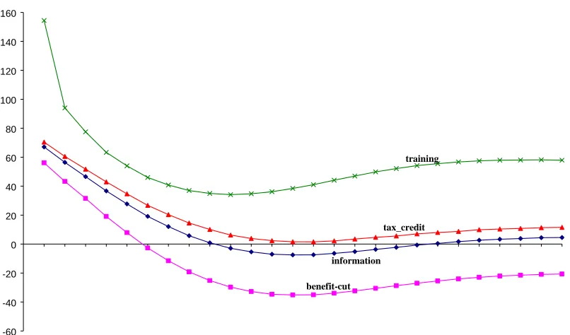
Results for displacement percentages from our four MONASH simulations are shown in Figure S1 and Table S1. Detailed explanations of these results are provided in section 4. The highlights are as follows.

• A training program may generate an abundance of inexperienced labour. This can cause large long-run displacement effects by reducing the wage rate available to non-target inexperienced workers.

• A training program may initially reduce aggregate employment, leading to a short-run displacement percentage of over 100 per cent.

• A benefit-cut program applied to a target group of long-term non-employed people may discourage some non-target people from voluntarily staying out of employment, leading to negative long-run displacement.

• As specified in our simulations, information and tax-credit programs have only minor effects on the income trade-off between work and non-work faced by people outside

2 _{These specifications are rather stylised. In future research it may be possible to provide a richer}

the target group. This leads to displacement paths that are consistent with simple theory.

In our applications of MONASH, we look at generic labour-market programs. We focus on big-picture effects, not fine detail. In future research it will be possible to add to MONASH the level of detail required to analyse particular real-world programs. The results presented here for generic programs suggest that analysis of particular programs will benefit from the dynamics, industry detail and economy-wide perspective of a general equilibrium model such as MONASH.3

Figure S1. Displacement percentages in MONASH simulations of four types of labour-market programs

-60 -40 -20 0 20 40 60 80 100 120 140 160

2006 2007 2008 2009 2010 2011 2012 2013 2014 2015 2016 2017 2018 2019 2020 2021 2022 2023 2024 2025 2026 2027 2028 2029 2030 2031 2032

information benefit-cut

tax_credit training

3 _{The importance of general equilibrium effects in the analysis of labour-market programs is also}

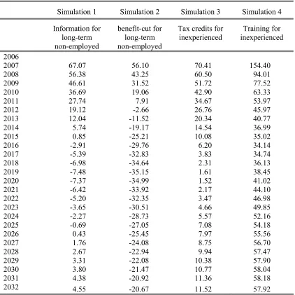
Table S1. Displacement percentages: data underlying Figure S1

Simulation 1 Simulation 2 Simulation 3 Simulation 4

Information for long-term non-employed

benefit-cut for long-term non-employed

Tax credits for inexperienced

Training for inexperienced

2006

2007 67.07 56.10 70.41 154.40

2008 56.38 43.25 60.50 94.01 2009 46.61 31.52 51.72 77.52 2010 36.69 19.06 42.90 63.33

2011 27.74 7.91 34.67 53.97

2012 19.12 -2.66 26.76 45.97

2013 12.04 -11.52 20.34 40.77

2014 5.74 -19.17 14.54 36.99

2015 0.85 -25.21 10.08 35.02

2016 -2.91 -29.76 6.20 34.14

2017 -5.39 -32.83 3.83 34.74

2018 -6.98 -34.64 2.31 36.13

2019 -7.48 -35.15 1.61 38.45

2020 -7.37 -34.99 1.52 41.02

2021 -6.42 -33.92 2.17 44.10

2022 -5.20 -32.35 3.47 46.98

2023 -3.65 -30.51 4.66 49.85

2024 -2.27 -28.73 5.57 52.16

2025 -0.69 -27.05 7.08 54.18

2026 0.43 -25.45 7.97 55.56

2027 1.76 -24.08 8.75 56.70

2028 2.67 -22.94 9.94 57.47

2029 3.31 -22.08 10.38 57.90

2030 3.80 -21.47 10.77 58.04

2031 4.38 -20.92 11.36 58.18

1. Introduction

1.1. Definitions

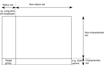
A labour-market program is a policy designed to increase the employment of a target group of non-employed people. As shown in Figure 1.1, the target group is the intersection of a subset of the potential labour force whose members have a particular non-employment status and a subset that has a particular characteristic. We refer to these subsets as the program’s status and characteristic sets. An example of a target group is long-term non-employed (status set) sole parents (characteristic set).

The displacement percentage of a labour-market program is an indicator of the extent to which the program generates a net increase in employment. The displacement percentage (D) is calculated for year t as:

D(t) ⎭ ⎬ ⎫ ⎩ ⎨ ⎧ ∆ − ∆ − ∆ − = t 1 t t 1 E E E *

100 (1.1)

where

t

E

∆ is the deviation in year t in total employment away from the basecase forecast caused by the program; and

t 1

E

∆ is the deviation caused by the program in the number of people in the target group in year t.

If the program succeeds in decreasing the target group by ten (-∆E_1t=10) but causes

aggregate employment (∆E_t=2) to increase by only two, then we say that the displacement

percentage is 80 per cent. The increase in aggregate employment may be restricted to two because eight target people obtained jobs that would have otherwise been taken by non-target people. Another possibility is that eight target people move to another category of non-employment.

Labour-market programs come in many forms. In this paper we look at four broad types:

(1) those that increase the ability of members of the target group to offer their labour services to employers by, for example, providing members of the group with

information concerning availability of jobs;

(2) those that aim to increase the supply of labour to employment activities by reducing the financial benefits of remaining non-employed to the target group;

(3) those that aim to increase the supply of labour to employment activities by increasing the after-tax wage rates that the target group can earn in employment by providing

(4) those that aim to increase the supply of labour to employment activities by increasing the after-tax wage rates that the target group can earn in employment by providing employment-relevant training.

Figure 1.1. Partitioning of the potential labour force

e.g. Long-term non-employed

Target group

Status set Non-status set

Characteristic set

Non-characteristic set

e.g. Sole parent

To quantify the effects of these types of labour-market programs, including displacement effects, we use an extended version of the MONASH model. MONASH is a dynamic computable general equilibrium (CGE) model of the Australian economy distinguishing about 100 industries (see Dixon and Rimmer, 2002). A MONASH simulation normally consists of two runs: a basecase forecast run and a policy run. In the basecase run for this paper, we establish business-as-usual forecasts for the years 2005 to 2030. In each policy run we develop an alternative forecast that includes the introduction of one of the four types of labour market programs. Comparison of a policy run with the basecase run shows the effects of a labour-market program as deviations from business-as-usual forecasts.

1.2. Literature

There is a vast literature on labour-market programs and displacement effects. Reviews include Martin (1998), Bartik (2000) and Kenyon (1994). In this literature there are four broad methods of assessing labour-market programs and calculating displacement effects: (1) demand and supply analysis; (2) probabilistic modelling; (3) econometric modelling; and (4) CGE modelling.

shift causes the intersection of demand and supply to move south-east. There is a reduction in the wage rate and an increase in aggregate employment. However the increase in aggregate employment is less than the increase in employment of the target group: displacement occurs because some previously employed people respond to the lower wage by withdrawing their labour services (there is movement down the supply curve). While demand and supply curves are a valuable starting point for organising thinking, more complete analysis requires several other ingredients including: non-homogenous labour; the specifics of particular labour-market programs; general equilibrium effects; and dynamics.

Some of these missing ingredients are captured by probabilistic modelling. This approach characterises labour-market programs as affecting the probability of a non-employed person entering employment. Piggott and Chapman (1995) provide an ingenious Australian application of probabilistic modelling in their analysis of the ‘Job Compact Program’ of the early 1990s. They capture specific features of the program and introduce dynamics.

As described by Piggott and Chapman, the Job Compact guaranteed employment for 9 months (1 period) to people who had been unemployed continuously for 18 months (2 periods). The Government created jobs for these people either directly (e.g. work in national parks) or indirectly by subsidizing businesses willing to employ them. Graduates from the program who failed to find a non-program job could re-enter the program after another two

periods of continuous unemployment

.

Econometric models provide another of the missing ingredients, non-homogeneous labour. They also allow for dynamics and some general equilibrium effects but are not strong on the specifics of labour-market programs. Bartik (2000 and 2002), for example, describes an econometric model in which there are 5 labour types. Using pooled times-series cross-section data from 50 U.S. states, he models state demands for labour of type i (ei) as a

function of the average wage rate in the state (w), the relative wage rate of i (wi/w) and

aggregate state income (y):

⎟

⎠

⎞

⎜

⎝

⎛

=

,

y

w

w

,

w

f

e

.

(1.2)

For each state, he models supply of labour of type i (lsi) as a function of: the wage rate of i;

income available to the unemployed (benefits); the unemployment rate for labour of type i (unempi); and a variable (shocki) used in simulating the effects of labour-market programs as

exogenous shifts in labour supply:

(

)

i g w ,benefits,unemp

ls = + shocki . (1.3)

Wage adjustments are modelled as functions of unemployment:

(

)

h

w_i = _i . (1.4)

Other equations introduce definitions of aggregates and define unemployment as the gap between employment and labour supply. Real world dynamics are introduced through lags in equations (1.2), (1.3) and (1.4) and general equilibrium effects are introduced by connecting income (y) to wages and employment.

In assessing a labour-market program, Bartik applies a positive value to shocki, where

i refers to the relevant target group (e.g. female head of household with low education). This generates an increase in lsi and a short-run increase in unempi. Via (1.4), there is a reduction

in wi leading to increase in ei. Bartik’s results imply that labour-market programs generate

significant short-run reductions in wages and high displacement. In the long run, both displacement and wage reductions are small.

functions and budget constraints of households. Against these strengths, CGE models often provide little in the way of dynamics4 _{and are only loosely tied to labour-market data.}

The model presented in this paper is of the CGE type. Following the CGE tradition, we assign values to key substitution parameters without estimation. However, we draw on key ideas from other approaches to labour-market modelling. Consistent with the demand and supply approach, we present a simple diagrammatic analysis. Consistent with the probabilistic approach, we represent labour-market programs as affecting the employment probabilities of different groups of labour-market participants. Consistent with the econometric approach, we include lags in our model through wage-adjustment equations and we attempt to trace out realistic dynamic paths.

1.3. Organisation

The paper is organized as follows.

In section 2 we describe the relevant aspects of the MONASH extension.

In section 3 we set up a stylized model in which the wage and investment dynamics are quite similar to those in MONASH. Our aim is to facilitate understanding of MONASH results on the effects of labour-market programs and particularly the results for the displacement percentage.

In section 4 we describe MONASH results on the effects of the four types of labour-market programs. Throughout section 4, we use ideas from the stylized model of section 3 to facilitate understanding of results from the much more complicated MONASH model. By using this approach, we expose the main mechanisms and assumptions responsible for our results without requiring readers to be familiar with MONASH.

Concluding remarks are in section 5.

2. Extensions of MONASH

2.1. Categories and activities

For studying labour-market programs, we created a version of MONASH in which the working-age population for year t is divided into ten categories, five for the set of people with the characteristic of a hypothetical program and five for the set of people without the characteristic. For each of these sets the five categories are:

4 _{Typically, CGE models generate results either for the short run (capital stocks fixed) or for the long}

(1) those who were employed in year t-1 (the working experienced category, Wc, c= 1 for

the characteristic subset and c= 2 for the non-characteristic subset)5_;

(2) those who were employed in year t-1 but employed in year t-2 (the short-run non-employed experienced category, SEc, c= 1, 2);

(3) those who were non-employed in year t-1 and not in the potential labour force in year t-2 (the short-run non-employed inexperienced category, SIc, c= 1, 2);

(4) those who were non-employed in year t-1 and in year t-2 (the long-run non-employed category, LNc, c= 1, 2); and

(5) those who were not in the potential labour force in year t-1 (the new entrant category, Nc, c= 1, 2).

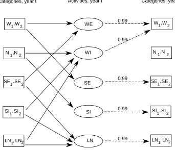
Each person in the potential labour force in year t participates in one of the following five activities:

(1) experienced work (activity WE); (2) inexperienced work (activity WI);

(3) short-run non-employment with recent work experience (activity SE); (4) short-run non-employment without recent work experience (activity SI); and (5) long-run non-employment (activity LN).

As indicated in Figure 2.1, people in categories W1 and W2 can participate in either

experienced work (activity WE) or short-run non-employment with recent work experience (activity SE). New entrants (categories N1 and N2) can participate in inexperienced

employment (activity WI) or short-run non-employment without recent work experience (activity SI). People in categories SE1 and SE2 can participate in either experienced work

(activity WE) or long-run non-employment (activity LN). Finally, people in categories SI1

and SI2 or LN1 and LN2 can participate in either inexperienced work (activity WI) or long-run

non-employment (activity LN).

The allocations of people from categories to activities (the dark arrows in Figure 2.1) are determined by:

(1) the demands by employers for experienced and inexperienced workers; (2) supply decisions by workers in different categories; and

(3) competition among people from different categories to fill vacancies in different activities.

5 _{As outlined in Appendix 1, we include 119 occupations in the extended MONASH model.}

Figure 2.1. Labour-market categories, activities and flows

W₁,W₂ WE

WI

SE

SI

LN

0.99

0.99

0.99

0.99

0.99

Categories, year t Activities, year t Categories, year t+1

1, 2

SE SE

1, 2

SE SE W

1,W2

N₁,N₂ N₁,N ₂

1, 2

SI SI

1, 2

SI SI

LN

1,LN2 LN1,LN2

2.2. Demand for labour

In modelling demands, we assume that at each point of time employers choose their labour inputs to maximize profits subject to a production-function constraint and a given availability of capital.6 _{This produces demand functions for labour by occupation (denoted by}

o) and experience (denoted by e) that reflect: the before-tax wage rates of experienced and inexperienced workers in different occupations; the availability of capital; and other relevant factors such as technology and product prices.

The production functions adopted in the extended version of MONASH have a nested CES form. The nesting allows: substitution between inputs of experienced and inexperienced labour in each occupation; substitution between inputs of different occupations; and substitution between inputs of labour and capital. Expressed in linear percentage-change form, the resulting demand functions for labour can be written as:

(

w

w

)

θ

*

w

w

(

w

;

k

;

a

....)

*

θ

d

⎟

+

Ω

⎠

⎞

⎜

⎝

⎛

₋

−

−

−

=

(2.1)

6 _{The capital stock adjusts through time via investment which is modelled as responding to changes in}

where

o

R

*

w

w

=

∑

= , (2.2)

and

j

_R

_*

_w

w

=

∑

= . (2.3)

In these equations

doej is the percentage change from year t-1 to t in industry j’s demand for labour of type

oe (occupation o, experience e);

oe

w is the percentage change in the real before-tax wage rate for an average7 _worker

in activity oe (assumed to be the same for all industries j);

oej

R is the share of labour of experience e in industry j’s costs of employing people in occupation o;

oj

R is the share of o in industry j's total labour costs;

j o

w

j

w is the percentage change to industry j in the overall real before-tax wage rate, defined in (2.3) as a share-weighted average of j

o

w

1

θ and θ₂ are positive parameters; and

Ωj is a function relating the percentage change in j’s overall demand for labour: to the

percentage change in the average real before-tax wage rate applying to workers in industry j; to growth in j’s capital stock (kj); to technical change (aoej) relevant to j’s use

of oe; and to other variables such as relative product prices.

The first term on the RHS of (2.1) allows industry j to substitute between inexperienced and experienced workers in the same occupation. In the simulations reported

in section 4, we set the experience-inexperience substitution elasticity (θ₁) at 2. Thus we

assume that employers are readily able to adjust the relative rates of growth in their labour forces of experienced and inexperienced workers in response to changes in relative wage rates.

The second term on the RHS of (2.1) allows industry j to substitute between workers

in different occupations. We set the substitution parameter θ₂ at 0.35, thereby assuming that

7 _{For most of this paper we assume that all oe workers receive that same before-tax wage rate.}

employers have only moderate scope to respond to changes in the relative costs of different occupations.

The last term on the RHS of (2.1) allows changes in the average wage payable by industry j to influence j's demand for labour through labour-capital substitution8_{. We also}

include in this last term capital growth and other non-wage variables that affect j's demand for labour.

2.3. Supply of labour

In modelling supplies, we assume that workers in each category solve a utility-maximizing problem in deciding how they would like to allocate their time between employment and non-employment and between different occupations. This produces offer- or labour-supply functions by each category of worker to each workforce activity that reflect relevant post-tax wage rates. For example, supplies by workers in the SE1 category reflect

post-tax wage rates available to characteristic workers for experienced employment and for long-run non-employment (long-run non-employment benefit rates to characteristic workers).

Specifically, we assume that at the beginning of year t, people in category q decide their labour-market offers for the year to n activities (covering occupations and non-employment) by solving a problem of the form: choose Lqc(t), c = 1, …, n to maximize

] L * B * AW ..., , L * B * AW [

U_{q q,1,t q,1,t q,1,t q,n,t q,n,t q,n,t} (2.4)

subject to n _q,t

1 c q,c,t

N

L =

∑

= (2.5)

where

Lq,c,t is the labour supply that people in category q plan to make to activity c in year t;

Nq,t is the number of people in category q in year t;

AWq,c,t is the real after-tax wage rate received by people in category q from labour in

activity c (if c is a non-employment activity, then AWqc(t) can be thought of as a real

benefit rate);

Bq,c,t is a taste variable -- increases in Bq,c,t impart a shift in the preferences of people in

category q in favour of spending time in activity c; and

Uq is a homothetic function with the usual properties of utility functions (positive first

derivatives and quasi-concavity).

Adopting a CES function for Uq, we obtained labour supply functions that can be

written in percentage-change form as follows:

8 _{In the MONASH simulations reported in this paper, we set the labour-capital substitution elasticities}

⎟ ⎟ ⎠ ⎞ ⎜ ⎜ ⎝ ⎛ + ∑ − + ε + =

= V *(aw b )

b aw

n n _{qg qg}

1 g qg qc qc q qc

l (2.6)

where

qc

l , nq, awqc and bqc are percentage changes between years t-1 and t in the variables

denoted by the corresponding uppercase symbols;

Vqg is the share of category q’s offers that are made to activity g ( Vqg = Lqg/Nq); and

ε is a positive parameter.

The value of ε controls group q’s substitution between different labour-market activities. In particular, ε influences the response of q’s labour-market choices to changes in

the relative wages (or benefits) between employment activities and non-employment. Thus, ε is an important determinant of the elasticity of labour supply from group q (defined as the percentage increase in q’s offers to employment for a one per cent increase in q’s average wage in employment activities relative to q’s benefits in non-employment). In setting a value for ε we ensured that the resulting economy-wide elasticity of labour supply was empirically realistic. For the simulations in section 4, we set ε = 2 which gave an economy-wide elasticity of labour supply of 0.12.9

In applications of MONASH that rely on (2.6), the starting values for the labour supplies Lqc play a critical role. Via these starting values we ensure only the flows allowed in

Figure 2.1 occur. Where q refers to new entrants (N1 or N2), short-term inexperienced

non-employed (SI1 and SI2) and long-term non-employed (LN1 and LN2), we ensure that all offers

to work are to inexperienced work activities by setting initial values for q’s offers to experienced work activities at zero. Where q refers to a short-term non-employed category (SI1, SI2, SE1 or SE2) we introduce a significant discouraged-worker effect by setting the

initial value of q’s offers to non-employment at 25 per cent of q’s total offers. Where q refers to a long-term non-employed category (LN1 or LN2) we introduce a strong

discouraged-worker effect by setting the initial value of q’s offers to non-employment at 50 per cent of q’s total offers. Where q refers to an employed category (W1 or W2) we ensure that all offers to

work are to experienced work activities by setting initial values for q’s offers to inexperienced work activities at zero. As explained in Dixon and Rimmer (2003), we also use the initial settings of the Lqcs to ensure that only realistic inter-occupational flows can occur.

For understanding the MONASH results in section 4, it is important to realize that only non-employed people (those in SE, SI and LN categories) make significant changes in

9 _{Labour-supply elasticities of this magnitude are consistent with those found by Kalb (1997). Details}

their offers to employment in response to changes in the after-tax wage rates they can earn in employment relative to the benefit they can receive in non-employment.

2.4. Determination of real before-tax wage rates, real after-tax wage rates and benefit rates

Before-tax wage rates payable for experienced and inexperienced work are modelled as adjusting sluggishly to gaps between supply and demand. If a policy causes the supply of a given type of labour to increase relative to demand, then we assume that the real before-tax wage rate of this type of labour falls in response to decreased worker negotiating strength.10

More precisely, we assume that

⎪⎭ ⎪ ⎬ ⎫ ⎪⎩ ⎪ ⎨ ⎧ −1 W W b t , oe p t , oe = ⎪⎭ ⎪ ⎬ ⎫ ⎪⎩ ⎪ ⎨ ⎧ − − − 1 W W b 1 t , oe p 1 t , oe + α ⎪⎭ ⎪ ⎬ ⎫ ⎪⎩ ⎪ ⎨ ⎧ − b t , oe p t , oe b t , oe p t , oe S S E E

for all employment activities oe (2.7)

In this equation:

the arguments oe denote an occupation and experience level. As indicated already, for the current MONASH application we have 119 occupations (see Appendix 1) and 2 experience levels (inexperienced labour, supplied by people from the N, SI and LN categories and experienced labour, supplied by people from the W and SE categories);

b t , oe

W is the real before-tax wage rate for an average worker in occupation o experience level e in year t in the basecase run;

b t , oe

E and S_oeb_,t are the employment and labour supply for occupation o experience level e

in year t in the basecase run -- Eb_oe,t is a sum over industries of demand for labour of type

oe and Sb_oe,t is a sum over categories of offers to oe;

p t , oe

W , Ep_oe,t and Sp_oe,t are the real before-tax wage rate, employment and labour supply for occupation o experience level e in year t in the policy run; and

α is a positive parameter.

Under (2.7), the real before-tax wage rate for oe in a policy run moves further above its value in the basecase run if the ratio of policy employment to basecase employment is greater than the ratio of policy labour supply to basecase labour supply. While labour-market programs

can temporarily produce gaps between the employment ratio (Ep_oe,t /Eb_oe,t) and the labour

supply ratio (Sp_oe,t/Sb_oe,t), we can expect these gaps to close under (2.7) as wage rates adjust

10 _{Our assumed wage-adjustment process is compatible with a search model [see for example,}

Bohringer et al. (2005)] in which increases in labour supply, and resulting increases in the

unemployment rate, generate increases in the value of having a job relative to the value of not having a job, thereby inducing workers to settle for lower wage rates. It is also compatible with efficiency-wage theory, see for example, Layard et al. (1994, pp. 33-45). Under this theory, employers offer wage rates

thereby bringing labour demand into line with supply. Our labour market specification can be summarised as short-run real-wage stickiness and long-run real-wage flexibility.

In both the basecase and policy runs, we relate the real after-tax wage rate that can be earned by people from category q for work in activity oe to the real before-tax wage rate of an average oe worker via the equation

(

)

t , oe , q k t , oe , q k t , oe k t , oe ,

q W *1 T *H

AW = −

for all employment activities oe and for k = b, p , (2.8)

where k t , oe , q

T is the tax rate in run k (basecase or policy) applying to wages earned by people from category q working in activity oe in year t; and

k t , oe , q

H takes the value 1 in most applications of our model but can be varied from 1 when we want to simulate the effects of training-induced differences in the productivity of oe workers from different categories with consequent differences in hourly wage rates.

Finally, we assume that the non-employed receive an exogenously set fraction of the average economy-wide average after-tax wage rate, that is

k t , g , q k t , ave k t , g ,

q AW *F

AW = for all non-employment activities g and for k = b, p , (2.9)

where k t , g , q

AW is the after-tax benefit received by people from category q in non-employment activity g in year t in run k;

k t , ave

AW is the average after-tax wage rate across work activities in year t in run k; and

k t , g , q

F is an exogenously set fraction.

2.5. Vacancies: determination of who gets the jobs

Under our sticky-wage specification, not all workers who offer their services to employment activities find jobs. This causes involuntary flows to non-employment activities. There are also voluntary flows to employment activities, especially from workers in non-employment categories. As mentioned earlier, we introduce discouraged-worker effects by modelling non-employed workers as offering large fractions of their potential labour services to non-employment activities.

remain in the activity. This applies to incumbents who wish to remain and to incumbents who wish to move to another employment activity but are unsuccessful in finding a vacancy.

The share of vacancies in each activity oe that are filled by non-incumbents from category q is q’s share of the non-incumbent offers to oe. Thus, for example, if a particular group of non-employed workers make 10 per cent of the non-incumbent offers to work activity oe, then they fill 10 per cent of the vacancies in oe.

3. Displacement in a simple dynamic model

In this section we introduce a stylized version of MONASH. We start in subsection 3.1 by setting up the model and describing the initial equilibrium. In subsection 3.2 we analyse the dynamic adjustment of employment and wages to a labour-market program. Subsection 3.3 describes the behaviour of the displacement percentage. At the end of subsection 3.3, we list conclusions from the stylized model that will be helpful in the analysis of results from MONASH.

3.1. The basecase, labour demand and the policy

For the stylized model, we assume that there is only one type of labour. Thus we simplify MONASH by ignoring the occupational and experience dimensions. We also ignore MONASH’s industrial dimension by assuming that there is a single industry.

Now refer to Figure 3.1. Assume that our basecase forecast is that the economy will stay perpetually at δ0, that is employment and the real wage rate will remain at E0 and W0 in

all years.11 _{Labour supply (people wanting to work) is permanently at S}

0: we draw the supply

curve vertically on the assumption that the wage rate for non-employment (e.g. benefits) is indexed to the wage rate for employment so that movements in the wage rate for employment do not affect the relative attractiveness to workers of employment and non-employment. Unemployment is fixed at S0 minus E0. At this level of unemployment we assume that there

is no pressure from the labour market to change the real wage rate.

We specify the labour demand function as:

) W ( g * K

E_t = _{t t} . (3.1)

where:

Et is employment in year t;

11 _{For the stylized model we assume that the basecase is a stationary equilibrium. As described in}

Figure 3.1. Dynamic adjustment of employment and wages under a labour-market program

W₀

North-West

∆Κ<0

∆W<0 ∆Κ<0

∆W>0

∆Κ>0

∆W<0

∆Κ>0

∆W>0

∆W=0

∆K=0

E₀ S₀ Ef Sf

D₀

D₀

hours

δ₀ δ_f

real wage

rate Df

D_f

North-East

South-West South-East

Kt is the capital stock in year t; and

g is a monotonically decreasing function of the real wage rate in year t, Wt.

In Figure 3.1 we have marked the demand curve for year 0 as D0D0.

Consistent with our assumption of a steady-state basecase, we assume that the rate of return on capital at δ0 is equal to the exogenously given world rate. This means that there is

no tendency for K to change from K0, which means that there is no tendency for the demand

curve for labour to move.

the employment level at which the rate of unemployment is the same as the initial rate is Ef,

where Ef satisfies

E0 /S0 = Ef /Sf . (3.2)

Given the shift in supply from S0 to Sf, how will the economy evolve from its initial

employment-wage point, δ0? To answer this question we consider the behaviour of the real

wage rate (W) and the capital stock (K) in the four quadrants of Figure 3.1 defined by the horizontal line through W0 and the vertical line through Ef.

3.2. The dynamic path of the employment-wage point

3.2.1. Wage behaviour (movement along the labour-demand curve)

Simplified so that it can be used in the context of Figure 3.1, the MONASH wage-adjustment specification [see (2.7)] is:

⎭ ⎬ ⎫ ⎩ ⎨ ⎧ −1 W W 0

t ₌

⎭ ⎬ ⎫ ⎩ ⎨ ⎧ − − ₁ W W 0 1

t _{+ α}

⎭ ⎬ ⎫ ⎩ ⎨ ⎧ − 0 t 0 t S S E E

, (3.3)

where

W0, E0 and S0 are the real wage rate, employment and labour supply in every year of the

basecase forecast;

Wt, Et and St are the real wage rate, employment and labour supply in year t with the

labour-market program in place (that is in year t of the policy run); and α is a positive parameter.

In the policy situation,

f

t S

S = for all t . (3.4)

Consequently, the wage rate will be decreasing from year to year in the policy run whenever

Et /E0 < Sf /S0 , (3.5)

that is

0 W<

∆ whenever E_t <E_f . (3.6)

Similarly,

0 W>

∆ whenever E_t >E_f (3.7)

and

0

W=

∆ when E_t =E_f . (3.8)

In terms of Figure 3.1, the real wage rate: is falling when we are in the North-West and South-West quadrants; is rising when we are in the North-East and South-East quadrants; and is stationary on the vertical line through Ef. At any given level of the capital stock (that is at any

employment-wage point along the labour-demand curve. This is indicated in Figure 3.1 by the direction of the ∆W arrows.

3.2.2. Capital-stock behaviour (movement of the labour-demand curve)

If the rate of return in year t (Rt) is greater than the initial rate of return (R0) then

Australia will attract capital inflow, causing the capital stock to increase and the labour-demand curve to move to the right. Similarly, if Rt is less than R0, then the capital stock will

decrease and the labour-demand curve to move to the left. To see what this means in terms of Figure 3.1, it is helpful to assume that Australia produces just one product, grain. Grain is used for consumption, exporting and as a capital good. We assume that producers hire units of capital up to the point at which the value of the marginal product of capital is equal to the rental rate, that is

⎟⎟ ⎠ ⎞ ⎜⎜ ⎝ ⎛ = t t t

t P *MPK K_E

Q , (3.9)

where:

Qt is the rent that must be paid by producers to the owners of capital for the use of a unit

of capital for one year; Pt is the price of grain; and

MPK is the marginal product of capital, which is a monotonically decreasing function of the ratio of capital input (Kt) to labour input (Et).

Ignoring various complications (e.g. taxes and depreciation) that are taken into account in MONASH but are inessential to the exposition presented here, we can represent the rate of return on investment in year t as the ratio of the rental on a unit of capital to the cost of a unit of capital (the ratio of the user price to the asset price). Since capital is made out of grain, the asset price is the price of grain (Pt). Thus, from (3.9) we see that

⎟⎟ ⎠ ⎞ ⎜⎜ ⎝ ⎛ = t t

t MPK K_E

R . (3.10)

Next we assume that the real wage rate in year t (Wt) equals the marginal product of labour

(MPL), that is

⎟⎟ ⎠ ⎞ ⎜⎜ ⎝ ⎛ = t t

t MPL K_E

W . (3.11)

MPL is a monotonically increasing function of the capital/labour ratio. Thus, we can conclude that

R_t <R₀, ∆K<0 and the labour-demand curve moves to the left whenever W_t >W₀

(3.13)

and

R_t =R₀, 0∆K= and the labour-demand curve is stationary when W_t =W₀ . (3.14)

In terms of Figure 3.1, the labour-demand curve: is moving to the right (∆K>0

)

)

horizontally. This is indicated in Figure 3. 1 by the direction of the K∆ arrows.

3.2.3. Dynamic path

Starting from δ0, the employment-wage point δt will be forced initially by

labour-market pressures to move down D0D0 into the South-West quadrant of Figure 3.1. Once δt is

in the South-West quadrant, labour-market and capital-market pressures combine to move it in a south-easterly direction (as indicated by the dotted line) until it reaches the vertical boundary through Ef. At this stage δt must pass into the South-East quadrant on a path with

zero slope (∆W=0 when E_t =E_f

).

In the South-East quadrant, δt must initially move in a north-easterly direction. While

δt is in the South-East quadrant, the wage rate rises. Eventually δt must leave the South-East

quadrant by arriving at the horizontal boundary through W0. It cannot leave the South-East

quadrant by crossing back into the South-West quadrant: if δt approached the vertical

boundary through Ef, then wage pressures would be negligible (∆W=0

)

pushed back into the South-East quadrant by capital pressures (∆K>0

)

There are two possibilities for δt’s departure from the South-East quadrant. The first

is that δt arrives directly at the new steady-state equilibrium, δf. This possibility is shown by

the dotted line in Figure 3.1. At δf the labour-demand curve DfDf is stationary: ∆K=0

because the rate of return is at its initial level. The wage rate is also stationary: the unemployment rate is at its initial level.

The second possibility is that the labour-demand curve overshoots its steady state position. In this case δt would cross into the North-East quadrant. It would then travel in a

north-westerly direction and cross into the North-West quadrant from where it would travel back into the South-West quadrant (its initial quadrant). In a sensibly parameterized model, δt

3.3. Behaviour of the displacement percentage

Assume that the population is made up of two groups, i = 1 and 2. Labour supply from group i is Li and the total supply of labour at time t is given by

t 2 t 1

t L L

S = + . (3.15)

Employment of the two groups is proportional to their supply, that is

t it

it

A

*

E

E

=

where

t it it L_S

A = for all t and i = 1, 2 . (3.17)

Underlying (3.16) and (3.17) is the assumption that each supplying worker has an equal chance of being employed, which implies that the share of group i in employment is the same as the share of group i in supply. Total employment is given by

t 2 t 1

t E E

E = + for all t . (3.18)

Assume that in the basecase, supply and employment for both groups are fixed at their initial values L10, L20, E10 and E20.

In the policy run, we introduce a labour-market program at time 0 targeted on not-employed people in group 1. Assume that the program causes a one-off increase in labour supply from group 1 but does not affect supply from group 2. In terms of Figure 3.1, all of the shift in supply from S0 to Sf is accounted for by a shift in supply from group 1. What will

happen to the displacement percentage, D(t), in the transition from δ0 to δf?

To answer this question, we derive an expression for D(t) as a function of the percentage deviations caused by the program in total labour supply and total labour demand.

We start by re-interpreting -∆E_1t in (1.1) as the deviation caused by the program in

the number of group-1 people who obtain jobs. (This is legitimate in our stylized model because we assume that the target group is all of the non-employed people in group 1.) Next, we divide the numerator and denominator of (1.1) by E0 to obtain

D(t) ⎭ ⎬ ⎫ ⎩ ⎨ ⎧ − = t 1 10 t t 1 10 e * A e e * A *

100 (3.19)

where e1t and et are the program-induced percentage deviations in employment of group 1 and

in total employment at time t and Ai0 is the basecase share of group i in total employment (and

in labour supply).

t t 1 t

1 a e

e = + for all t , (3.20)

where a1t is the program-induced percentage deviation in A1t from its basecase value. From

(3.17) we obtain

t t 1 t

1 s

a =_l − for all t , (3.21)

where _l1tand st are the program-induced percentage deviations at time t in supply by group 1

and in total supply. Noting that the supply of group 2 is fixed, we use (3.15) to give

t 1 10

t A *

s = _l for all t . (3.22)

By combining (3.20), (3.21) and (3.22) we find that

t 10 t 20 t 1

10*e A *s A *e

A = + for all t . (3.23)

Now we use (3.23) to eliminate e1t from (3.19). This yields

D(t)

(

)

⎭ ⎬ ⎫ ⎩ ⎨ ⎧ + − = t 10 t 20 t t 20 e * A s * A e s * A *

100 (3.24)

Formula (3.24) reveals the following:

• If et is zero, then displacement is 100 per cent. This means that displacement will be

high in the early years of a labour-market program. In terms of Figure 3.1,

displacement is high when we first move away from δ0.

• Displacement falls towards zero as et approaches st. In terms of Figure 3.1, this

means that displacement declines from 100 per cent towards zero as δt moves

south-east through the South-West quadrant.

• Displacement is zero when et = st. In terms of Figure 3.1, this means that

displacement reaches zero when δt reaches the vertical boundary through Ef.

Equivalently, displacement is zero when the deviation in the real wage rate reaches its largest negative percentage value.

• Displacement is negative when et is greater than st. In terms of Figure 3.1, this means

that displacement becomes negative when δt crosses into the South-East quadrant. If

δt moves directly to δf from the South-East quadrant (as illustrated by the dotted line

in Figure 3.1), then displacement will converge to zero from below. If δt moves to δf

along a converging spiral, then displacement will asymptote to zero with damped oscillations between positive and negative values.

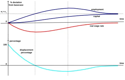
expectations are summarized in Figure 3.2. In Figure 3.2 we adopt the dotted path in Figure 3.1 and draw stylized paths showing the effects of a labour-market program on employment, capital and the real wage rate together with the implied path for the displacement percentage. Where MONASH results differ from those expected on the basis of the stylized model, we need to look for and assess the mechanisms in MONASH that cause the differences.

Figure 3.2. Effects of a labour-market program in a stylized model

time time employment

capital real wage rate

displacement percentage e = s_{f f}

% deviation from basecase

percentage 100

0 0

4. Effects of four types of labour market programs: results from the MONASH

model

4.1. Provision of job information to a subset of the non-employed

In our first simulation the status set is the long-term non-employed. We include among the long-term non-employed not only those who are actively looking for work but also those who are discouraged. Discouraged workers believe that there are no jobs available that would be suitable for them.

For the characteristic set we simply take a representative 10 per cent of the potential labour force. For discussion purposes, it is convenient to think of the characteristic set as being the left-handers. In the first year of our simulation (2007), we assume the proportions of characteristic and non-characteristic people are the same across the W, N, SE, SI and LN categories. For example, we assume that the number of people in W1 is 10 per cent of the

but does not apply in policy runs. In policy runs the relative labour-market positions of characteristic and non-characteristic people is affected by the labour-market program under consideration.

The target group (the intersection of the status and characteristic sets) is the long-term non-employed left-handers. We assume that the target group can provide inexperienced labour services that are identical to those that can be provided by other suppliers of these services. In other words, we assume that the distinguishing characteristic of the target group is unobserved or irrelevant to employers.

The labour-market program that we examine in the first simulation is improved information provision to the target group. We assume that such a program encourages people in the target group to apply for jobs by causing a shift in their preferences towards work activities and away from non-employment activities. We represent these preference shifts as 5 per cent shocks in 2007 to a subset of the Bq,c,t’s appearing in the utility function (2.4). The

shocks are administered in the policy run via (2.6) with the inclusion among the shocks for 2007 of:

bq,c = 5 for all categories q in the target group and for all employment activities c. (4.1)

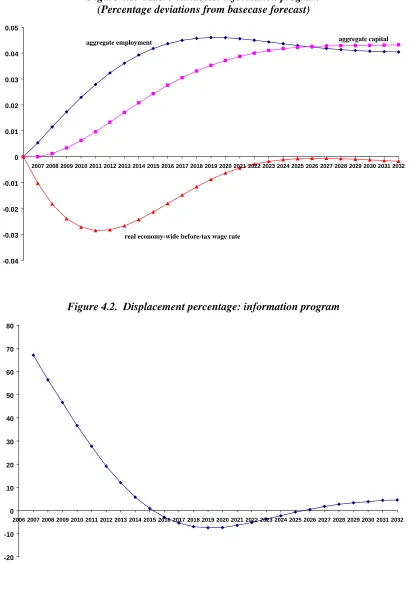
MONASH results generated under (4.1) are shown in Figures 4.1 to 4.4. With the exception of the displacement percentage in Figure 4.2, all results are expressed as percentage deviations between variable values in the policy and basecase runs.12 _{Thus, for example, the}

result in Figure 4.1 for 2014 for aggregate employment means that the information program implemented in 2007 causes employment in 2014 to be 0.04 per cent higher than it would have been in the absence of the program.

The results in Figures 4.1 and 4.2 are highly compatible with those from our stylized model (compare Figures 4.1 and 4.2 with Figure 3.2). As in Figure 3.2, in Figures 4.1 and 4.2,

• employment and capital show approximately equal percentage long-term deviations;

• the capital deviation rises steadily to its long-term value;

• the employment deviation rises strongly, overshoots and then moves back to its long-term value;

12 _{The displacement percentage is defined according to (1.1). It is meaningful only in policy runs.}

• the deviation in the average economy-wide real before-tax wage rate becomes increasingly negative, reaches a trough and then returns in the long-run to approximately zero;

• the employment deviation peaks and the displacement percentage troughs in the same year (2019); and

• the path of the displacement percentage declines from a high value, crosses through zero, troughs and then turns up towards zero.

The main differences between the MONASH results in Figures 4.1 and 4.2 and the stylized results in Figure 3.2 concern the displacement percentage. In Figure 4.2:

(a) the displacement percentage passes through zero (about 2015) well after the average real before-tax wage rate troughs (2011) or equivalently, the displacement percentage is positive when the wage rate troughs; and

(b) the displacement percentage asymptotes in the long run above zero rather than at zero.

As we will see below, the feature of MONASH that causes (a) is endogeneity of labour supply and the feature that causes (b) is our treatment of severances.

4.1.1. Why is the displacement percentage positive when the real before-tax wage rate troughs?

In the stylized model, we assumed that the supply of labour to employment is completely exogenous (the supply curves in Figure 3.1 are vertical). The labour-market program simply causes an exogenous increase in offers to employment from the target group and no change in the offers from the non-target group. By contrast, in MONASH the labour-market program can affect offers to employment endogenously. It does this by altering wage rates and causing changes in offers to employment not only by people in the target group but also by people outside that group.

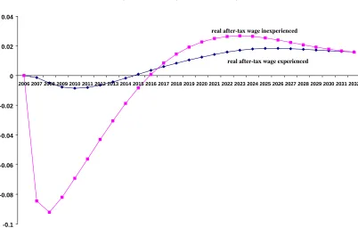
As can be seen from Figure 4.3, under shock (4.1) there is an immediate reduction in the real before-tax wage rate of inexperienced workers relative that of experienced workers. This reflects the initial increase in the supply of inexperienced labour from the left-handed long-term non-employed. In terms of equation (2.7), shock (4.1) causes an immediate

increase in Sp_oe,t/Sb_oe,t for all oe where oe is an inexperienced work activity.

rate moves with the average after-tax wage rate [see (2.9)]. The increase in the benefit rate relative to the wage rate for inexperienced employment causes a reduction in offers to employment by non-target people who can offer inexperienced labour (particularly categories SI1, SI2 and LN2, see Figure 2.1). This means that the overall increased level of supply to

employment is comprised of an increase in the supply by the target group and a slightly offsetting decrease in supply by the non-target group.

Thus in the policy simulation, at the point of no wage pressure when the percentage increase in supply is matched by the percentage increase in employment, there is a positive deviation in employment of the target group and a slightly negative deviation in employment of the non-target group. Consequently, at this point (when the wage rate troughs), the displacement percentage is positive.

4.1.2. Why does the displacement percentage asymptote above zero in the long run?

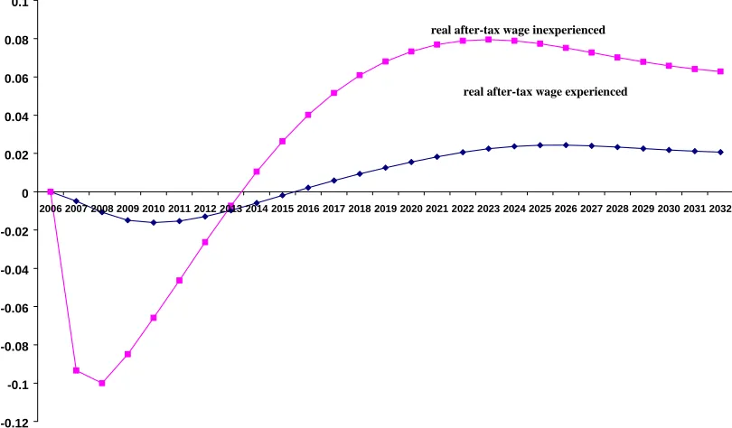
The information program has a long-run positive effect on aggregate employment, thereby increasing the aggregate supply of experienced workers and decreasing the number of long-term non-employed workers. Despite reducing the number of long-term non-employed workers, the program has a positive effect on aggregate supply of inexperienced labour: the increase in supply per left-handed long-term non-employed person happens to more than offset the decrease in the number of long-term non-employed people. It happens in the long run that the percentage increases in the supplies of inexperienced and experienced workers are approximately matched. Thus, as can be seen from Figures 4.3 and 4.4, the long-run deviations in the wage rates (in either before- or after-tax terms) of experienced and inexperienced workers are approximately the same.

This means that there are no long-run incentives for non-target people to shift their offers between employment and non-employment activities. So why is the displacement percentage positive in the long run, implying a negative deviation in employment of non-target people?

4.2. Reducing benefits to a subset of the non-employed

As in the first simulation, in the second simulation the target group is the left-handed long-term non-employed. The labour-market program is reduced benefits for this group. We introduce the program to the policy run in 2007 by setting:

fq,g = -5 for all categories q in the target group and for all non-employment activities g,

(4.2)

where fq,g is the percentage change between 2006 and 2007 in F_qp_,g,t appearing in (2.9). The

aim of the program is to induce the target group to offer more strongly to employment activities by increasing the income that they can earn from employment relative to the income that they receive from non-employment.

MONASH results generated under (4.2) are shown in Figures 4.5 to 4.8. As in the first simulation, the results in Figures 4.5 and 4.6 are highly compatible with those from the stylized model. Again, the main differences between the MONASH results and the stylized results concern the displacement percentage. This time the displacement percentage in the MONASH results asymptotes in the long run below zero rather than at zero.

The programs in both the first and second simulations can be thought of as working primarily through an outward shift in the supply-to-work curve of left-handed long-term non-employed people. However, the benefit-cut program has two additional effects. First, it directly changes the supply incentives of left-handed short-term non-employed people. It induces them to increase their offers to employment and reduce their offers to non-employment (where they would receive a reduced benefit). Second, as can be seen from Figure 4.8, the benefit-cut program causes a long-run increase in the real after-tax wage rate of inexperienced workers relative to experienced workers. This in turn causes a further reduction in the benefit/wage ratio for all non-employed people who could potentially offer

inexperienced labour. Thus in the long run, the benefit-cut program causes an increase in offers to employment and ultimately an increase in employment of people in target non-employment categories. This allows the increase in aggregate non-employment to exceed the increase in employment of target people, explaining the negative long-run displacement percentage.

Why does the benefit-cut program cause a long-run increase in the real after-tax wage rate of inexperienced workers relative to experienced workers whereas this wasn’t the case in the information program (compare Figures 4.8 and 4.4)? The answer lies mainly in the supply response of short-term experienced non-employed left-handers (SE1). In the

to experienced employment. This has the effect of increasing the inexperienced/experienced wage ratio in the benefit-cut program relative to that in the information program.

We turn now to the short run. As for the information program, the benefit-cut causes a short-run increase in the supply of inexperienced labour relative to experienced labour. This results in an initial reduction in the inexperienced/experienced wage ratio calculated in both before- and after-tax terms (Figure 4.7 and 4.8). By applying the argument in subsection 4.1.1, we can explain why the displacement percentage is positive in the benefit-cut program at the point where the real before-tax wage rate troughs.

4.3. Provision of tax credits for inexperienced employment

The status set for our third simulation is the inexperienced non-employed, that is the people who can potentially supply inexperienced labour (people in the N, SI and LN categories, Figure 2.1). As in the previous two simulations, the characteristic set is the left-handers. Consequently, the target group consists of the people in N1, SI1 and LN1.

The labour-market program that we examine is the provision of tax credits paid to the target group on earnings from inexperienced employment. The program is represented in the policy run by including among the shocks for 2007:

(1) negative shocks to T_qp_,oe,t in (2.8) for e = inexperienced, q belongs to the target group and all occupations o; and

(2) offsetting positive shocks to T_qp_,oe,t for e = experienced and inexperienced, q belongs to the non-target group and all occupations o. The offsetting shocks generate the tax revenue necessary to finance the tax-credits paid to the target group.

As with the benefit-cut program, the aim of the tax-credit program is to induce the target group to offer more strongly to employment activities by increasing the after-tax income they can earn from employment relative to the income they receive from non-employment.

MONASH results for the tax-credit program are shown in Figures 4.9 to 4.12. Once again, the results are highly compatible with those from our stylized model (compare Figures 4.9 and 4.10 with Figure 3.2). As with the previous two programs, the main differences between the MONASH results and the stylized results concern the displacement percentage. The displacement path in Figure 4.10 has the same shape as that in Figure 3.2 but is moved up the page. In Figure 4.10, the displacement path does not cross zero and asymptotes in the long run well above zero. For understanding the position of the displacement path in Figure 4.10, it is necessary to look at the incentives that the tax-credit program gives to all

By providing tax credits, the program sharply increases the after-tax wage rate that the target group can earn in employment (Figure 4.11). It has only small indirect effects on all other after-tax wage rates from employment (Figure 4.12).13 _{Thus the tax-credit program}

increases the tax wage rate for employment of the target group relative to all other after-tax wage rates for employment. With the benefit rate being an average of after-after-tax wage rates for employment, the benefit rate falls relative to the after-tax wage rate for employment of the target group and rises relative to the after-tax wage rates for employment of all non-target people. Thus the program increases offers to employment by the target group and ultimately increases their employment. But at the same time, the program reduces the incentive to supply labour for all non-target non-employed people. This produces a strong displacement effect, explaining the elevated position on the page of the displacement path in Figure 4.10.

Why isn’t the displacement effect even higher: why isn’t it above 100 per cent? Offers to employment by the target group are sensitive to changes in the group’s after-tax-wage/benefit ratio. By increasing this ratio, the program generates a significant increase in supply from the target group. On the other hand, offers to employment by most people in the workforce (the employed) are insensitive to changes in their after-tax-wage/benefit ratio. Thus for most non-target groups, the reduction on this ratio has little effect on supply. This allows the program to generate a net increase in labour supply and therefore in employment, keeping the displacement percentage well below 100 per cent.

4.4. Provision of training to a subset of the non-employed

The status, characteristic and target sets in our fourth simulation are the same as those in the third simulation. Here we simulate the effects of providing all left-handed inexperienced non-employed people (those in the N1, SI1 and LN1 categories) with

employment-relevant training. We assume that the training enables these people, if they gain employment, to increase the number of units of output that they can produce per hour of work by 5 per cent. This enables them to earn 5 per cent more per hour than untrained inexperienced workers. From the point of view of employer incentives, there is still no difference between using left- or right-handed inexperienced labour. As with the tax-credit and benefit-cut programs, the training program aims to increase the offers to employment of the target group by increasing the wage that they receive from employment relative to the benefit that they receive from non-employment.

13 _{In looking at Figures 4.11 and 4.12, note that they are drawn with different scales on the vertical}