The Immersed Interface Method for Two Dimensional Helmhotlz / Poisson Equation with Complex Number Space.

ABSTRACT

ZHANG, SIDONG MAX. The Immersed Interface Method for Two Dimensional Poisson / Helmholtz Equations in Complex Number Space. (Under the direction of Dr. Zhilin Li.)

This thesis describes an expanded Immersed Interface Method for solving the

two-dimensional Helmholtz /Poisson equations in the complex number space with an interface.

Across the interface, the coefficient of the Helmholtz equation may have a finite

discontinuity, and the source term of the Helmholtz /Poisson equations can have singular

source terms. The solution and its normal derivatives can have discontinuities across the

interface. Then we apply the developed method for solving Helmholtz /Poisson equations on

irregular domains using the augmented immersed interface method.

This dissertation utilizes a combination of methodologies including the immersed interface

method, Fast Fourier Transformation algorithm, augmented strategies, least squared

interpolations, and the Generalized Minimal Residual method (GMRES) in complex number

space for the Schur complement system. This expanded IIM is structured that the computed

solutions are second order convergent towards the exact solution. Moreover, the cost of

computation is designed to be efficient when solving the Schur complement system with

almost constant number of iterations.

This dissertation also includes numerical experiments that have two different type problems.

The results have confirmed the theoretical analysis expectation. The computed solutions

showed statistically second order convergence. The proposed method is efficient, robust for

The Immersed Interface Method for Two Dimensional Helmholtz/Poisson Equations in Complex Number Space

by

Sidong Max Zhang

A dissertation submitted to the Graduate Faculty of North Carolina State University

in partial fulfillment of the requirements for the degree of

Doctor of Philosophy

Applied Mathematics

Raleigh, North Carolina

2013

APPROVED BY:

_______________________________ ______________________________

Dr. Zhilin Li Dr. Alina Chertock

Committee Chair

________________________________ ________________________________

ii

DEDICATION

iii BIOGRAPHY

Mr. Sidong Max Zhang was born in Shanghai, China, 1965. He attended

middle-school and high-middle-school at No.1 High School Affiliated to East China Normal University,

where he was first inspired by mathematics, science, and computer programming. Upon

graduating from Shanghai University of Science and Technology with a BS in Applied Math

in 1988, he worked in Shanghai Soap Factory as a statistician and dispatcher for three years.

Mr. Zhang matriculated in Wake Forest University in 1991, and graduated with a

Master of Arts degree in Math two years later. Then he survived as a statistical and

sometimes IT consultant for about ten years working in various companies, there he earned

some valuable interpersonal skill and experience, including the ability of listening and

talking to different kinds of people.

Accidentally, Mr. Zhang found his passion for teaching mathematics. He began to

pursue his Ph.D. degree at North Carolina State University in 2008, and expecting to

iv

ACKNOWLEDGMENTS

It is my honor to thank the many people who have helped me through this work.

First and foremost, I am very grateful for having Dr. Zhilin Li as my thesis advisor

and mentor. He provided me with precise research scholarship, invaluable guidance, and vast

knowledge for my Ph.D study. Whenever he traveled the world and no matter the time zone,

I could always rely on email or Skype to talk to him for academic assistance, support, and

encouragement. Dr. Li had profoundly improved my way of doing mathematics. Our

friendship became much more than just teacher and pupil.

Besides my advisor, I would like to sincerely thank the rest of my thesis committee:

Dr. Xiaobiao Lin, Dr. Alina Chertock, and Dr. Roger McGraw for their encouragement,

insight, and knowledge. Dr. Lin also taught my Real and Functional Analysis courses, and

the analytical skills that I learned from him will impact me far beyond this dissertation. Dr.

McGraw is more than just a teacher to me, because he has given me so much advice in

academics and real life that I will benefit forever.

I will always look back on my education with fond memories of the professors and

staff at NCSU. Dr. Putch, Dr. Schacter, Dr. Flup, and Dr. Tran are among the best teachers

that any student can have. Thanks to Ms. Denise Seabrook for helping me with all of my

v

I am so fortunate to have Peng Song, GuanYu Chen, Gady and Ranya as my

academic brothers/sister. Bonded with the knowledge of Immersed Interface Method, we

shared the hard struggle and the sweet joy of success together.

I would also like to thank Ms Heather Manhart, Mr. Brian Tew, and Dr. Yu-Mong

Hsiao for proof- reading this dissertation. Their suggestions and comments have not only

made the sentences flaw more smoothly, but also added some vivid color to the language.

Thanks to Dr. Meredith Williams, who has verified the statistical analysis, especially the

linear regression models about convergence and their hypothesis tests, which is totally

irreplaceable for proving 2nd order convergence.

Last but not least, I would like to thank my family for the unselfish support

emotionally and financially. My dear wife Ching, daughter Lily, and son Chris have

constantly reminded me to do my “homework”. I can always count on Lily for words and

spelling, she is better and faster than any software checking package. Chris helped me on the

computers, printers, and networks. My in-laws, He YangYuan and Lu YunFang have always

been firmly believed in my ability and success. And all this would not be possible without

vi

TABLE OF CONTENTS

LIST OF TABLES ……….…... ix

LIST OF FIGURES ………..……….…..… xi

CHAPTER 1. Introduction ……… 1

1.1 The Application Problem ……….……… 2

1.2 Helmholtz and Poisson Equations ………... 4

1.3 Review of Existing Numerical Methods ………. 6

1.3.1 Immersed Boundary Method ……… 6

1.3.2 Integral Equation Method ………. 8

1.3.3 Immersed Interface Method ……….. 9

1.4 Outline of the thesis ……… 10

CHAPTER 2. ZFFT methods for solving two dimensional Poisson / Helmholtz Equations in Rectangular Domains ……..………. 12

2.1 ZFFT Method with hx ≠ hy, and m = n ………. 13

2.2 ZFFT Method with hx = hy, and m ≠ n ………. 15

2.3 ZFFT Method with hx ≠ hy, and m ≠ n ………. 18

2.4 ZFFT Method Summary ……… 20

2.5 Efficiency Analysis ……… 20

vii

CHAPTER 3. Immersed Interface Method for Two dimensional Poisson / Helmholtz

Equations in Complex Number Space ………..………... 25

3.1 Interface Embedding ……….………. 25

3.2 Local Coordination Transformation ……….. 27

3.3 Interface Relations ………. 29

3.4 The Finite Difference Scheme of the IIM ……….. 31

3.5 Correction Terms at Irregular Grid Points ………. 32

CHAPTER 4. Augmented Strategies ………... 36

4.1 The Augmented Variable ………... 37

4.2 Discrete System of Equations in Matrix-Vector Form ……….. 37

4.3 Least Squared Interpolation ………... 38

4.4 Schur Complement System ……… 42

4.5 GMRES for the Schur Complement System ……….……... 43

CHAPTER 5. Numerical Experimental Results ………..………... 45

5.1 Numerical Example 1 ……… 50

5.2 Numerical Example 2 ……… 61

viii

CHAPTER 6. Conclusions ……….. 75

6.1 Research Conclusions ……… 75

6.2 Future Research Work ………... 76

REFERENCES ……… 77

APPENDICES …..………... 82

Appendix A PROLOGUE OF THE PACKAGE fft_poisson_complex3 ………… 83

ix

LIST OF TABLES

Table 5.1a Grid Refinement Analysis for Example 5.1.1 .….………...………... 51

Table 5.1b More Grid Refinement Analysis for Example 5.1.1 .….……….………... 51

Table 5.2 Convergence Analysis for Example 5.1.1 ………... 53

Table 5.3a Grid Refinement Analysis for Example 5.1.2 ………..………..… 54

Table 5.3b More Grid Refinement Analysis for Example 5.1.2 ………..… 54

Table 5.4 Convergence Analysis for Example 5.1.2 ………... 56

Table 5.5a Grid Refinement Analysis Example 5.1.3 ………..………...… 57

Table 5.5b More Grid Refinement Analysis Example 5.1.3 ………..…..………...… 57

Table 5.6 Convergence Analysis for Example 5.1.3 ………... 59

Table 5.7 Computing Cost Analysis: Number of Iteration for Example 5.1.1 ……… 60

Table 5.8 Computing Cost Analysis: Number of Iteration for Example 5.1.2 ……… 60

Table 5.9 Computing Cost Analysis: Number of Iteration for Example 5.1.3 ……… 60

Table 5.10a Grid Refinement Analysis for Example 5.2.1 ………..………... 62

Table 5.10b More Grid Refinement Analysis for Example 5.2.1 ………... 62

Table 5.11 Convergence Analysis for Example 5.2.1 ………. 64

Table 5.12a Grid Refinement Analysis for Example 5.2.2 ………..……….….. 65

Table 5.12b More Grid Refinement Analysis for Example 5.2.2 ……….….. 65

Table 5.13 Convergence Analysis for Example 5.2.2 ………. 67

Table 5.14a More Grid Refinement Analysis for Example 5.2.3 …………..………..….. 68

x

Table 5.15 Convergence Analysis for Example 5.2.3 ………. 70

Table 5.16 Computing Cost Analysis: Number of Iteration for Example 5.2.1 ………….. 71

Table 5.17 Computing Cost Analysis: Number of Iteration for Example 5.2.2 ………….. 71

Table 5.18 Computing Cost Analysis: Number of Iteration for Example 5.2.3 ………….. 71

xi

LIST OF FIGURES

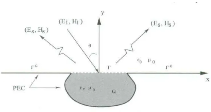
Figure 1.1 A Diagram of an Electromagnetic Wave Model ………..….………….…….. 2

Figure 1.2 A Rectangular Domain with an Embed Interface ……….….……... 3

Figure 3.1 A Solution Domain and an Embed Interface ……….…... 25

Figure 3.2 Interface, Regular and Irregular Points ………….……….…….. 28

Figure 3.3 An Irregular Grid Point, its Orthogonal Projection, and Local Coordinates .. 29

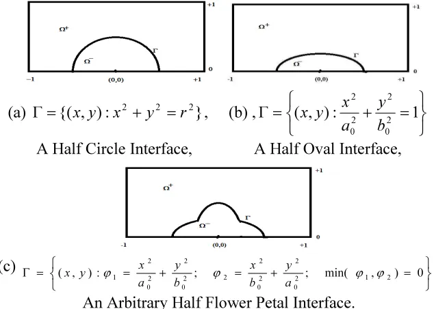
Figure 5.1 Domains and Interfaces. (a) A Half Circle Interface, (b) A Half Oval Interface,

(c) An Arbitrary Half Flower Petal Interface ………... 49

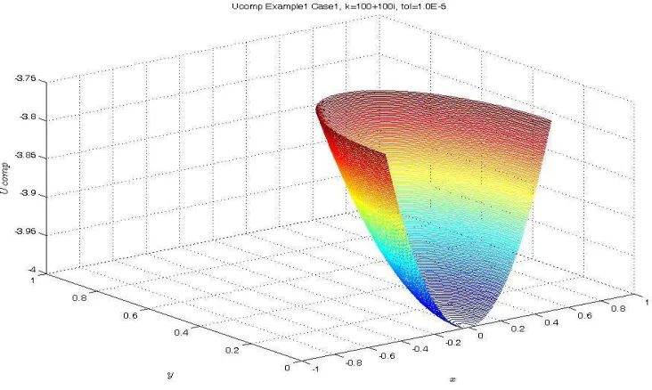
Figure 5.2. Computed Solution for Problem One with A Half Circle Interface,

k=100+100i, m=256, n=128 ………. 52

Figure 5.3. Error of Computed Solution for Problem One with A Half Circle Interface,

k=100+100i, m=256, n=128 ………. 52

Figure 5.4 Convergence Order Comparison for Problem One with A Half Circle

Interface ……….... 53

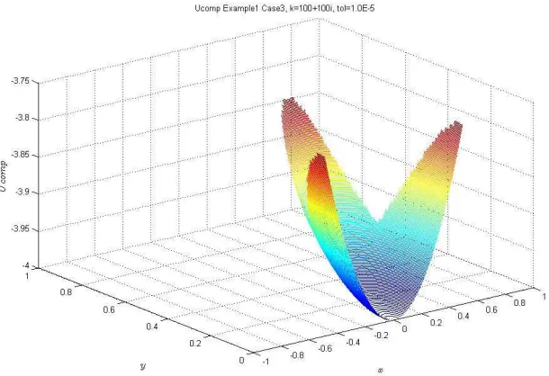
Figure 5.5. Computed Solution for Problem One with A Half Oval Interface,

k=100+100i, m=256, n=128 ……… ……….…..……… 55

Figure 5.6. Error of Computed Solution for Problem One with A Half Oval Interface,

k=100+100i, m=256, n=128 ……….………. 55

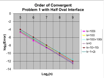
Figure 5.7. Convergence Order Comparison for Problem One with A Half Oval

xii

Figure 5.8. Computed Solution for Problem One with An Arbitrary Flower Petal

Interface, k=100+100i, m=256, n=128 ……….………... 58

Figure 5.9. Error of Computed Solution for Problem One with An Arbitrary Flower Petal

Interface, k=100+100i, m=256, n=128 …..………. 58

Figure 5.10 Convergence Order Comparison for Problem One with An Arbitrary Flower

Petal Interface ………..……… 59

Figure 5.11 Computed Solution for Problem Two with A Half Circle Interface,

k=100+100i, m=256, n=128 ……… ………. 63

Figure 5.12. Error of Computed Solution for Problem Two with A Half Circle Interface,

k=100+100i, m=256, n=128 ……….……..………. 63

Figure 5.13 Convergence Order Comparison for Problem Two with A Half Circle

Interface ……….………..……… 64

Figure 5.14. Computed Solution for Problem Two with A Half Oval Interface,

k=100+100i,m=256, n=128 ………..………... 66

Figure 5.15. Error of Computed Solution for Problem Two with A Half Oval Interface,

k=100+100i, m=256, n=128 ……….………... 66

Figure 5.16 Convergence Order Comparison for Problem Two with A Half Oval

Interface ………... 67

Figure 5.17. Computed Solution for Problem Two with An Arbitrary Flower Petal

Interface, k=100+100i, m=256, n=128 ……….……..……… 69

Figure 5.18. Error of Computed Solution for Problem Two with An Arbitrary Flower

xiii

Figure 5.19 Convergence Order Comparison for Problem Two with An Arbitrary Flower

1

CHAPTER 1

Introduction

In this dissertation, we studies two-dimensional Helmholtz Equation in complex number

space in general irregular domains with a Dirichlet boundary condition:

2 2

2 2 2 ( , ), ( , )

( , ) 0, ( , )

( , ) : ; ( , ) : ; .

u u

ku f x y x y R

x y

u x y x y

where u x y C f x y C k C

∂ ∂

+ + = ∈ Ω ⊂

∂ ∂

= ∈ ∂Ω

Ω → Ω → ∈

(1.1)

These particular equations are used describe many problems related to steady-state

oscillations in different media, such as mechanical, acoustical, thermal and electromagnetic

phenomena. These problems also have been widely used in military and civil engineering

communities.

In reality of the electromagnetic field models, the domains are more than likely to have

discontinuous media with general irregular interfaces, and the models may have a complex

wave number (k) which represents both electric and magnetic charges. These phenomena

present extra challenges for the researchers and engineers, because the traditional methods

are usually designed for rectangular domains, and real wave numbers. This dissertation is

2

1.1 The Application Problem and its Difficulty

Developed by Maxwell and Hertz, the theory describing electromagnetic waves can be

written in the format of Helmholtz equation [14,27].

For example in [9,43], Figure 1.1, demonstrates the electromagnetic scatting from a

two-dimensional open cavity filled with inhomogeneous media. The ground plane and the walls

of the open cavity are assumed as perfect electric conductors (PEC), and the interior of the

open cavity is filled with non-magnetic materials which may be inhomogeneous. The half

space above the ground plan is filled with a homogenous and isotropic medium with its

permittivity ε and permeability µ. Also, the electromagnetic scattering by the cavity is

governed by the Helmholtz equation along with Sommerfeld’s radiation conditions imposed

at infinity.

3

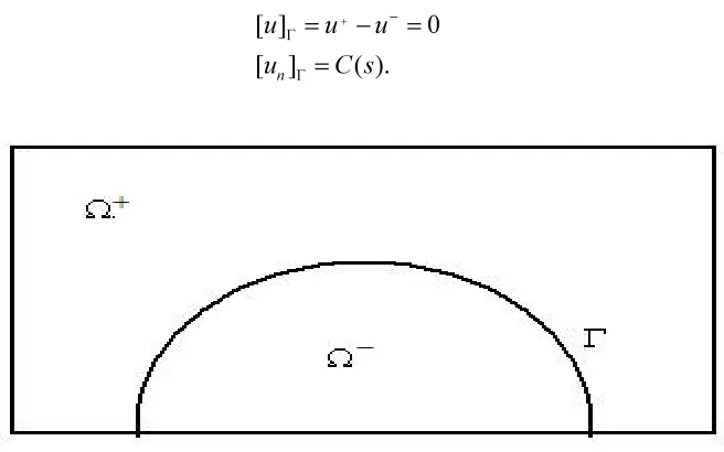
Due to difficulties in designing the finite difference approximations close to a curved

boundary, the irregular domain will be embedded into a larger rectangle domain. So, the

original differential equation is extended to the rectangular domain correspondingly by

introducing the following jump conditions across the interface, where the interface Γ is the

boundary of the original domain.

[ ] 0

[ ] ( ). n

u u u u C s

+ −

Γ Γ

= − =

=

Figure 1.2 Rectangular Domain with An Embed Arbitrary Interface.

Therefore, the harmonic Maxwell equation is reduced to Helmholtz equation format:

.

, ) , ( ,

0

, ) , ( ), , (

0 2 0εrµ k k where

y x u

y x y

x f ku u

− =

Ω ∈ =

Ω ∈ =

+ ∆

+ −

Another advantage of embedding an irregular domain into a rectangular domain is that it is

4

1.2 Helmholtz and Poisson Equations

The Helmholtz equation in rectangular domain has the following form

Φ − = +

∆u ku _{. (1.2)}

The particular two-dimensional Helmholtz equation in the Cartesian coordinate system:

) , ( 2 2 2 2 y x f ku y u x u = + ∂ ∂ + ∂ ∂

, (1.3)

where k is the wave number (in some reference, it is expressed as k2

); f is a source. To

simplify our notation, we write the right-hand as f(x, y) instead of −Φ(x, y) in this

dissertation. If k=0, then (1.3) became a Poisson equation:

) , ( 2 2 2 2 y x f y u x u = ∂ ∂ + ∂ ∂

. (1.3a)

For a homogeneous Helmholtz equation with f≡0, the general analytic solution exists, and

can be written as a combination of following particular solutions

. ), sinh cosh )( sinh cosh ( . ), sin cos )( sinh cosh ( . ), sinh cosh )( sin cos ( . ), sin cos )( sin cos ( 2 2 2 1 2 2 1 1 2 2 2 1 2 2 1 1 2 2 2 1 2 2 1 1 2 2 2 1 2 2 1 1 µ µ µ µ µ µ µ µ µ µ µ µ µ µ µ µ µ µ µ µ µ µ µ µ − − = + + = + − = + + = − = + + = + = + + = k y D y C x B x A u k y D y C x B x A u k y D y C x B x A u k y D y C x B x A u (1.4)

For inhomogeneous Helmholtz equation in the rectangle domain (say 0 ≤ x ≤ a, 0 ≤ y ≤ b),

with Dirichlet boundary condition as prescribed:

). ( ) , ( ), ( ) 0 , ( ), ( ) , ( ), ( ) , 0 ( 4 3 2 1 x f b x u x f x u y f y a u y f y u = = = = (1.5)

The solution for Helmholtz problem exists if ( ); 1,2,... 1,2,...

2 2 2 2 2 = = +

≠ n m

b m

a n

5

The solution can be written analytically in an integral equation involving Green’s function

. )] , , , ( )[ ( )] , , , ( )[ ( )] , , , ( )[ ( )] , , , ( )[ ( ) , , , ( ) , ( ) , ( 0 4

0 3 0

0 2

0 1 0

0 0

∫

∫

∫

∫

∫ ∫

= = = = ∂ ∂ − ∂ ∂ + ∂ ∂ − ∂ ∂ + = b b b b a b a b d y x G f d y x G f d y x G f d y x G f d d y x G f y x u ξ η ξ η ξ ξ η ξ η ξ η η ξ ξ η η η ξ ξ η ξ η η ξ η ξ η η ξ ξ

where the Green’s function G(*) has the following forms of representation:

, ) , ( ) sinh( ) sin( ) sin( 2 ) , , , ( ) , ( ) sinh( ) sin( ) sin( 2 ) , , , ( 1 1

∑

∑

∞ = ∞ = = = m m m m m m n n n n n n x Q a q y q b y x G or y H b p x p a y x G ξ µ µ ξ η ξ η β β ξ η ξ where , , , , 2 2 k q b m q k p a n p m m m n n n − = = − = = µ π β π and    ≤ ≤ ≤ − ≤ ≤ ≤ − =    ≤ ≤ ≤ − ≤ ≤ ≤ − = . 0 , )] ( sinh[ ) sinh( , 0 , )] ( sinh[ ) sinh( ) , ( , 0 , )] ( sinh[ ) sinh( , 0 , )] ( sinh[ ) sinh( ) , ( a x for b x a x for x a x Q b y for b y b y for y b y H m m m m m n n n n n ξ ξ µ µ ξ µ ξ µ ξ η η β β η β η β η

Though, we can analytically give out the solution for rectangular domains and

boundary condition [41], they will become very complicated and not practical for physics

and engineering use when the domain is general and irregular. Thus, numerical methods and

6

1.3 Review of Existing Numerical Methods

For a problem defined on an irregular domain, the method most often used is the

embedding technique. We will discuss in detail later in chapter 3 and 4 of this dissertation.

Then the problem can be treated as a special interface problem. Therefore, the terminology of

interface problems is introduced to include the problems defined on irregular domains.

There are many algorithms and methods discussed in research papers in the literature

that address the interface problem. For example, smoothing method for discontinuous

coefficients, harmonic averaging for discontinuous coefficients, immersed boundary method,

numerical integral equation method, ghost fluid method, and immersed interface method are

the most frequently referenced in the related fields. This dissertation just focus on the two

dimensional method that has closest relation to our algorithm, that is the Immersed Boundary

method, the numerical integral equation method, and existing Immersed Interface Method.

1.3.1 Immersed Boundary (IB) method

This Immersed Boundary method was originally developed by Peskin [29, 30, 31, 32,

33] to model the blood flow in a human heart, and has been applied to many other problems,

7

One of the most important ideas in the IB method is the use of a discrete delta

function to distribute a singular source to nearby grid points. The commonly used discrete

delta functions in one dimension are as following.

Hat delta function

   ≥ < − = . | | , | | , 0 , / |) | ( ) ( 2 ε ε ε ε δ ε x x if if x x

Cosine delta function

    ≥ < + = . 2 | | , 2 | | , 0 ), 2 cos( 1 ( 4 1 ) ( ε ε ε π ε δ ε x x if if x x

And Radial Delta function

. 2 | | , 2 | | , | | , , 0 4 | | 12 7 | | 2 5 8 1 , 4 | | 4 1 | | 2 3 8 1 ) ( 2 2 2 2 ε ε ε ε ε ε ε ε ε ε ε ε δ ε ≥ < ≤ <                       − + − − −         − + + − = x if x if x if x x x x x x x

In two dimensions, the discrete delta function often is the product of one dimensional

discrete delta functions, such as δε(x,y)=δε(x)δε(y). And the discretized Helmholtz

equation at (xi, yj) became

, ) ( ) ( * * , 1

, ij h i i h i i ij k k j j i i

ku ku x x y y f

s

k

k + = − −

∑

=

+

+ δ δ

8

where ks is the number of discrete points {(xi*, yj*)} on the interface, {γk}’s are the

coefficients that involved in the finite difference scheme, h is the mesh spacing. In this way,

the singular source is distributed to nearby grids points in a neighborhood of the interface Γ.

The Immersed Boundary method is robust and simple to implement. It has been

applied to many problems in mathematical biology and computational fluid mechanics [1, 2,

4, 5, 7, 8, 10, 11, 12, 39, 42, 44]. Various work has been developed to improve the accuracy

of the IB method, and it is most time first order convergence results [29, 31,30], with some

occasional second order convergence [17, 34]. But, there is not yet any complete analytical

convergence proof for the IB method [30]. However, stability analysis of the IB method is

given in [37, 38] for a membrane problem.

1.3.2 Integral Equation Method

Greenhaum, Mayo and their collaborators [23, 24, 25, 26] are among the few who

first combined integral equation based on the single and double layer theory with finite

difference methods to solve a Poisson equation on an irregular domain. The irregular domain

is embedded into a larger rectangle, and then the problem is recast as an elliptic interface

problem such that the solution is harmonic in the rectangle, excluding the boundary. Taylor

expansions at irregular grid points and the integral representation of the particular solution

near the irregular boundary are used. The source strength is determined from an integral

9

the finite difference schemes at all grid points in the rectangular domain so that a fast Poisson

solver can be used.

By solving the integral equation and a regular Poisson equation, the algorithm is

somehow second order accuracy in L∞ _{norm. The numerical integral equation methods are}

most effective for homogeneous source terms and certain boundary conditions. Although this

method still can be applied for nonhomogeneous source terms and different boundary

conditions if with some extra effort. The implementations of these methods, especially when

they are coupled with the fast multipole method, are difficult.

1.3.3 Immersed Interface Method

Immersed Interface Method is first developed by LeVeque and Li in 1994 [19]. It is

motived by Peskin’s IB method, but there are remarkable improvements in IIM. IIM is a

sharp interface method which the discontinuities or the jump condition are enforced exactly

by prior knowledge or approximately through Augmented strategy [20, 16].

In general cases, standard finite difference methods are used in discretization. At the

grid point near or on the interface, a correction term is added according to the jump condition

to ensure point-wise convergence. By this approaching, IIM can still take advantage of

existing numerical algorithm to solve the differential equation system. In most cases, IIM can

10

This dissertation is trying further expending Immersed Interface Method into

complex-numbered wave number and function, while thus preserving its advantages, like

efficient and stable solution with second order convergence.

1.4 Outline of the thesis

Chapter One surveys the general IIM background and literature. The fundamental

concepts such as interface problems and jump condition are introduced. The last section

describes the structure of this thesis.

In Chapter Two, we studied the solution for Poisson and Helmholtz equations in

rectangular domains without interface jump conditions. A new Fast Fourier Transformation

method is derived and analyzed for the efficiency and stability.

In Chapter Three, we introduced correction terms at irregular grid points such that the

proposed algorithm is 2nd order convergence.

In Chapter Four, we further studied some unknown interface conditions. Augmented

Strategies are used to assume one of the unknown interface variables, and estimated by

weighed least square interpolation, then we created Schur complement system. Finally,

11

Two examples of numerical experiments are presented in Chapter Five. Under

different functions, interface condition and computing circumstances, all results are in line

with our previous analysis.

The last chapter summarizes the contributions we have achieved and discusses

several possible future research topics.

At the end of the thesis is a list of papers, books and presentations which this research

12

CHAPTER 2

ZFFT methods for solving two dimensional Poisson /

Helmholtz Equation in Rectangular Domains

The Fast Fourier Transformation (FFT) method for solving two dimensional Poisson’s

equations was first introduced by Cooley and Tukey [15] in 1965. It was focused on squared

domains with uniformed mesh space. The main idea of this method is to take advantage of

some beautiful properties of the discrete Fourier transformation, which is able to decompose

the tridiagonal matrix into multiplication of eigenvalues and their eigenvectors. Therefore, by

substituting the variables back and forth twice, the FFT method only needs O(NlogN)

multiplications instead of computing the inverse of the matrix, thus it is much faster.

In 1984, Swarztrauber further developed the FFT method for rectangular domains [40]. He

first converted the two-dimensional solution ui,j into 1-dimensional vector umi+j, and turned

the finite difference scheme into a tridiagonal block matrix, and then solve the linear

equations system using row reduction method. This method achieved O(NlogN) (N=m×n)

efficiency. But it is somehow confusing, and not easy to understand and implement.

To ensure the efficiency of our computing, the FFT method in this dissertation is designed

for rectangular domains. For inscribing an arbitrary shape into another geometry shape, a

rectangular is more than likely to cover less area than a square. Thus the rectangular

13

In addition, we also need double complex precision for our data to keep rounding errors from

distorting our computing result. For example, we need the Schur complement residues in

very high precision so that the jump condition in the interface can be accurately obtained.

However, there is no existing FFT method that fit for our requirements at the time. Besides,

modern day computing environment is completely different from the 60s to 80s, the old

Fortran code that developed at that time may be obsolete and may not be complied smoothly

nowadays. So, we decided to develop our very own Fast Fourier Transformation methods for

rectangular domains with double complex precision. We would like to call the new algorithm

ZFFT, it is because this Fast Fourier Transformation method is dealing with complex number.

There three slightly variation of the algorithms total, we are going to introducing them one by

one.

2.1 ZFFT Method with hx

≠

hy, and m = n

First, we consider the discrete finite difference equation for Poisson equation in a rectangular

domain with the standard 5 point finite difference scheme at a rectangular domain can be

written as

n j

i f h

u u

u

h

u u

u

ij

y

ij j

i j i

x

ij j i j i

, , 1 , , 2

2

2 1 , 1 , 2

, 1 , 1

L

= ≈

− +

+ −

+ _{− + −}

14

where hx and hy are the mesh spaces in their respect x-axis and y-axis direction, and we

assume that hx ≠ hy, and m = n. Notice that fi,j is the right hand side value intergraded with

boundary condition. To rewrite (2.1) in matrix format

F UT h TU h y x ≈ + ₂ 2 1

1 _{, (2.2)}

where

(

i j

)

_nn

(

ij

)

_nn

n n f F u U and T , , , , , , 2 0 0 0 0 2 1 0 0 1 2 1 0 0 1 2 = =                 − − − − = L M O M M M L L L .

Apply discrete Fourier Transformation to each column of T, then T=V-1DV. (2.2) became

(

)

. ... 1 , , ) ) 1 ( 2 ( sin 4 , 0 0 0 0 0 0 , ) ) 1 ( 2 2 sin( , , 2 12 1 , , , 2 2 1 2 1 2 n j i n i D n ij S S V where F h h DV UV h DVU V h i n j i n n j i y x x y = + − =               = + = = = + − − π λ λ λ λ π K M O M M K K (2.3)

It is worth to point out that V has another beautiful property that

V n V 1 2 1 + =

− . (2.4)

Multiply hx2hy2, and V from left and V-1 from right to (2.3) at both sides, then

1 2 2 1 2 1

2 − − −

=

+h VUV D h h V FV

DVUV h

y x x

y . (2.5)

Now, let U VUV 1 u_{i,j n,n}

) (

=

= − , and F hxhyVFV fi,j n,n

1 2 2 ) ( =

= − , then

F D U h U D h x

y + =

2 2

15

Since D is diagonal matrix, then Ū in (2.5) can be easily solved

n j

i where h

h f u

j x i y

j i j

i , , 1K

2 2

,

, =

+ =

λ

λ . (2.7)

Further, for Helmholtz equation, (2.7) can be

n j

i where k

h h h

h

f u

y x j x i y

j i j

i , , 1K

2 2 2

2

,

, =

+ +

=

λ

λ . (2.8)

Once we have Ū, then reverse discrete Fourier Transformation,

V U V U −1

= . (2.9)

This Fast Fourier Transformation method is directly derived from the traditional

method for square domain. The tridiagonal matrix T is n×n square matrix. However, we

estimate the locate truncation error through (2.1), we can find out that it may not guaranteed

to be second order convergence for the computed solutions. So we keep on working on the

next method.

2.2 ZFFT Method with hx = hy, and m

_≠

n

In this method, we still start the finite difference equation for Poisson equation in a

rectangular domain with the standard 5 point finite difference scheme. This time, the mesh

16

grid points in that 2 direction are not equal (n ≠ m). It can be written as

n j m i f h u u u h u u u ij ij j i j i ij j i j i , , 1 ; , , 1 , 2 2 2 1 , 1 , 2 , 1 , 1 L L = = ≈ − + + − + _{− + −}

+ _{. (2.10)}

Notice that fi,j is the right hand side value intergraded with boundary condition. Rewrite (2.10)

in matrix format

F h UT U T n m 2 =

+ , (2.11)

where

( )

,

( )

. , 2 0 0 0 0 2 1 0 0 1 2 1 0 0 1 2 , 2 0 0 0 0 2 1 0 0 1 2 1 0 0 1 2 , , , , , , n m j i n m j i n n n m m m f F u U T T = =                 − − − − =                 − − − − = L M O M M M L L L L M O M M M L L L (2.12)

By discrete Fourier Transformation, Ts= Vs-1DsVs, s = m, n, then

F h V D UV U V D V n n n m m m 2 1 1 = + −

− _{. (2.13)}

Again, Multiplying h2, Vm from left and Vn-1 from right at both sides of the (2.13), we have

1 2

1

1 − −

−

=

+ m n n m n

n m

mV UV V UV D h V FV

D _{. (2.14)}

Let n m j i n mUV u

V

U 1 _{, ,}

) (

=

= − , and F h VmFVn fi,j m,n

1 2 ) ~ ( ~ =

= − . (2.15)

Then substitute (2.15) into (2.14), it become

F D U U D n m ~ =

17

Since Dm and Dn in (2.16) are diagonal, we can simply solve (2.16) for Ū,

n j

m i

f

u _n

j i m

j i j

i , 1, , ; 1, ,

~

) ( ) (

,

, = L = L

+ =

λ

λ . (2.17)

Similarly, for Helmholtz equation

n j

m i

k h f

u _n

j i m

j i j

i , 1, , ; 1, ,

~

2 ) ( ) (

,

, = L = L

+ +

=

λ

λ . (2.18)

Reverse the discrete Fourier transformation, we get

n

mUV

V U −1

= . (2.19)

This method uses traditional equal mesh spacing, while the numbers of grid points are

different in x-axis and y-axis direction. It is most compliable with the traditional numerical

analysis, and we can still take advantage of many existing software packages. In this method,

we have to construct two different set of discrete Fourier Transformation in (2.13), which

cost little extra computing. When it was used iteration like GMRES, we can store and re-use

them rather constructing from new each time. More important, the locate truncation error can

be estimated as usual, which we will prove later that it is second order convergence for the

computed solution against exact solution. So we decided to use this ZFFT II method for the

18

2.3 ZFFT Method with hx

≠

hy, and m

≠

n

For the completeness of this academic exploration, we want to further study the method with

rectangular mesh spacing and unequal number of grid points. Let us consider discrete

Poisson equation with, hx ≠ hy and m ≠ n, then

. , 1 ; , , 1 , 2 2 2 1 , 1 , 2 , 1 , 1 n j m i f h u u u h u u u ij y ij j i j i x ij j i j i L L = = = − + + − + − + − + (2.20)

Notice that fi,j is the right hand side value intergraded with boundary condition. Rewrite (2.20)

as matrix format, then

F UT h U T h n y m x ≈ + ₂ 2 1

1 _{, (2.21)}

where Tm and Tn are defined in (2.12)

Apply discrete Fourier Transformation to each column of Ts , i.e.

m m m

m V D V

T −1

= , and Tn Vn DnVn 1 −

= , (2.22)

(

)

). ) 1 ( 2 ( sin 4 , 0 0 0 0 0 0 . ... 1 , , ) ) 1 ( 2 2 sin( , 2 ) ( ) ( ) ( 2 ) ( 1 ) ( , , ) ( , + − =               = = + = = n i D n j i n ij S S V where n i n n n n n n j i n n n j i n π λ λ λ λ π K M O M M K K

Then, we have

F h h V D UV h U V D V h y x n n n x m m m y 2 2 1 2 1 2 = + −

19

Now, Multiplying hx2hy2, Vm from left and Vn-1 from right for both sides of (2.23), then

1 2 2 1 2 1

2 − − −

=

+ x m n n x y m n

n m m

yD V UV h V UV D h h V FV

h _{. (2.24)}

Let n m j i n mUV u V U , , 1 ) ( =

= − , and F hxhyVmFVn fi,j m,n 1 2 2 ) ˆ ( ˆ =

= − , (2.25)

then (2.24) become

F D U h U D

h_y2 _m + _x2 _n = ˆ . (2.26)

Since Dm and Dn are diagonal, it is easy to solve (2.26) for Ū,

n j m i h h f u _n j x i m y j i j

i , 1, , ; 1, ,

ˆ ) ( 2 ) ( 2 ,

, = L = L

+ =

λ

λ . (2.27)

Similarly, for Helmholtz equation,

n j m i k h h h h f u y x n j x i m y j i j

i , 1, , ; 1, ,

ˆ 2 2 ) ( 2 ) ( 2 ,

, = L = L

+ +

=

λ

λ . (2.28)

Once we have Ū, then by the reversed discrete Fourier Transformation (2.19), it is easy to get

the solution U.

This third ZFFT method is the combination of ZFFT method I and ZFFT method II. It is a

generalized algorithm that solves Poisson or Helmholtz equation. In practice of this research,

it is an over kill to simulate the rectangular shape by both measures of rectangular grid shape

and unequal mesh size. However, somebody may need this method for future research

20

2.4 ZFFT Method Summary

We mainly focus on the second complex-numbered Fast Fourier Transformation method

(ZFFT II) in rectangular domain for this summary. Other methods in this chapter are almost

identical. Here is the step by step approaching of the algorithm

1. Perform discrete Fourier Transformation on F, get

n m n

m _n V FV

h FV V h F 1 2 2 1 2 + =

= − . (2.29)

2. Compute middle solution Ū:

n j m i k h f u _n j m i j i j

i , 1, , ; 1, ,

2 ) ( ) ( ,

, = L = L

+ + =

−

λ

λ , (2.30)

where .

) 1 ( 2 sin 4 , ) 1 ( 2 sin

4 2 ( ) 2

) (       + − =       + − = n j m i n j m i π λ π λ

3. Perform reversed discrete Fourier Transformation on Ū, get

n m n

mUV _m V UV

V U 1 2 1 + =

= − . (2.31)

2.5 Efficiency Analysis

From previous section, we can see that the cost of step Two is 3×m×n operation, and step

21

straightforward matrix multiplication method, then the cost is m×m×n+ m×n×n flops, which

is O(m3_{). However, the triple matrix multiplication actually represents the Discrete Fourier}

Transformation. Thus, we can use convolutions and recursive algorithm, therefor the

computation cost is reduce the (m2

log2m) [6]. Here is the process for VmFVn as an example.

Let Fj={f1j,f2j, … , fmj}T be the the jth column of the F matrix, and

. 1 , ) 1 2 sin( ) 1 2 cos( , ) ( 1 2 2 3 2 1 − = + ⋅ − + = = + + + + = + − i m i m e where f f f f a m i m mj j j j π π ω ω ω ω ω π L (2.32)

ω is also known as a principal (m+1)th root of unity. The DFT of Fj is just the polynomial

(2.32) evaluation at the points {ω0, ω1, ω2, …, wm-1}. Conversely, the inversed DFT is the

polynomial interpolation producing the coefficients of a polynomial given its values at {ω0,

ω1, ω2, …, wm-1}.

Assume m=2s , then we divide the polynomial (2.32) into two equal pieces.

). ( ) ( ) ( ) ( ) ( 2 2 4 6 2 4 2 4 5 2 3 1 2 3 2 1 ω ω ω ω ω ω ω ω ω ω ω ω even odd j j j j j j m mj j j j a a f f f f f f f f f f a ⋅ + = + + + + + = + + + + = L L L (2.33)

From above, to evaluate two polynomials aodd and aeven of degree m/2-1 at (ωj)2 . But this is

really just m/2 points ω2j for 0 ≤ j ≤ m/2−1 since 2 2( 2)

m j

j +

=ω

ω . Thus evaluating a

polynomial of degree m-1=2s-1 at all m (m)th roots of unity is the same as evaluating two

22

multiplication additions. This can be done recursively with following algorithm

end y return y a y y a y a DFT y a DFT y a a a a a a a a a a e a return then n if a size n a DFT function even T odd even even T odd odd even even odd odd n even n odd n n r r r r r r r r r r r r r L r L r L r r r r ⋅ − = ⋅ + = = = = = = = = = − − ω ω ω ω ω ω ω ω π ) ( ) ( ) , , , ( ) , , , ( ) , , , ( 1 ); ( ) ( 6 4 2 1 5 3 1 1 2 / 2 1 0 ) / 2 (

Therefore, the computing cost of each column of a m×n matrix is

2 3

log₂ m_⋅ m, and by same

method, the cost of each row of each column of a m×n matrix is

2 3

log₂n n

⋅ . So, the total

computing cost for a m×n matrix is O

(

m_⋅n_⋅log(m_⋅n)

)

. The recursive method requires huge

memory for stocking of heap, which was not available in the 6os or 80s. Also for small

number mesh size, there are no significant different from recursive method compare to direct

matrix multiplication.

2.6 Error Analysis

Since we have u(x, y): R2

C, then we can write

23

First, let us consider the locate truncation error (LTE) for the standard 5-point finite

difference scheme for real function v(x,y) at grid point (xi, yj).

2 , 1 , 1 , , 1 , 1 2 2 2 2 ₄ ) ( ) ( h v v v v v v y x v

LTE _ij i j i j ij i j i j

− + + + − ∂ ∂ + ∂ ∂

= + − + − _{, (2.34)}

where i=1,…, m; j=1,…, n, and vij =v(xi, yj) . By Taylor expansion;

). ( ) ( ! 4 1 ) ( ! 3 1 ) ( 2 1 ) ( ), ( ) ( ! 4 1 ) ( ! 3 1 ) ( 2 1 ) ( ), ( ) ( ! 4 1 ) ( ! 3 1 ) ( 2 1 ) ( ), ( ) ( ! 4 1 ) ( ! 3 1 ) ( 2 1 ) ( 5 4 , 4 4 3 , 3 3 2 , 2 2 , , 1 , 5 4 , 4 4 3 , 3 3 2 , 2 2 , , 1 , 5 4 , 4 4 3 , 3 3 2 , 2 2 , , , 1 5 4 , 4 4 3 , 3 3 2 , 2 2 , , , 1 h O h v y h v y h v y h v y v v h O h v y h v y h v y h v y v v h O h v x h v x h v x h v x v v h O h v x h v x h v x h v x v v j i j i j i j i j i j i j i j i j i j i j i j i j i j i j i j i j i j i j i j i j i j i j i j i + ∂ ∂ + ∂ ∂ − ∂ ∂ + ∂ ∂ − = + ∂ ∂ + ∂ ∂ + ∂ ∂ + ∂ ∂ + = + ∂ ∂ + ∂ ∂ − ∂ ∂ + ∂ ∂ − = + ∂ ∂ + ∂ ∂ + ∂ ∂ + ∂ ∂ + = − + − + (2.35)

Substitute (2.35) into (2.34), and simplify

) ( ) ( ) ( 12 1 )

( ₄ 3 2

4

4 4

2 _{O h O h}

y v x v h v

LTE _ij + =

∂ ∂ + ∂ ∂

= _{. (2.36)}

By the same method, we can have the locate truncation error for w

) ( ) ( ) ( 12 1 )

( ₄ 3 2

4

4 4

2 _{O h O h}

y w x w h w

LTE _ij + =

∂ ∂ + ∂ ∂

= _{. (2.37)}

24 ). ( ) ( ) ( 12 1 ) ( ) ( 12 1 ) ( ) ( 12 1 ) ( ) ( 12 1 ) ( ) ( 12 1 ) ( ) ( 12 1 | ) ( ) ( | ) ( 2 2 1 4 4 4 4 2 1 4 4 4 4 2 2 3 4 4 4 4 2 2 3 4 4 4 4 2 3 4 4 4 4 2 3 4 4 4 4 2 h O h O y w x w i h O y v x v h h O y w x w h i h O y v x v h h O y w x w h i h O y v x v h wi LTE i v LTE u

LTE _{ij ij j}

=       + ∂ ∂ + ∂ ∂ +       + ∂ ∂ + ∂ ∂ =       + ∂ ∂ + ∂ ∂ +       + ∂ ∂ + ∂ ∂ =       + ∂ ∂ + ∂ ∂ + + ∂ ∂ + ∂ ∂ = ⋅ + = (2.38)

Furthermore, T is diagonally dominant, thus the global error is O(h2) for Poisson

equations. Very similar for Helmholtz equation, if the exact solution exists, i.e.

. , , 1 ; , , 1 , ) ( ) ( 2 n j m i k

h ≠−λ_im −λ_jn = L = L (2.34)

25

CHAPTER 3

Immersed Interface Method for Two dimensional Poisson

/ Helmholtz Equation in Complex Number Space

In this chapter, we try to develop an improved finite difference scheme to handle the

discontinuous f and coefficients cross the interface in complex number space. The real

number two-dimensional elliptic interface problem was solved using immersed interface

method [20]. Our approach is also based on immersed interface method, and very similar to

the real number one. The goal of our approach is to obtain a finite difference scheme that

works with discontinuous f and second order convergence guaranteed.

3.1 Interface Embedding

Let Ω be a convex domain in two dimensions within there is an irregular interface Γ. Let Ω+

and Ω- be the two regions of the interface, see following Figure 3.1.

26

We are considering the following Helmholtz / Poisson problem

Ω =

+

+Uyy kU f in

Uxx , . (3.1)

With some boundary condition on ∂Ω and jump conditions on the interface Γ.

w u u

u ₌ + ₋ − ₌

Γ

]

[ . (3.2)

g n u

n u

u_n =

∂ ∂ − ∂ ∂ =

− +

Γ

]

[ . (3.3)

In this study, we assume that the interface Γ is arbitrarily smooth, Ω is piecewise

smooth, k and f are piecewise continuous in Ω+ and Ω- respectably, and along the interface,

w has continuous second derivatives and q has continuous first derivatives. Then the solution

u has piecewise second order derivatives components in Ω, that is u ∈ C2 _in

Ω+ or Ω-, but not

in Ω .

Since the f and/or k may be discontinuous across the interface, the solution and its

derivatives may also be non-smooth or even discontinuous across the interface. Therefore the

traditional standard finite difference schemes will not work properly for this class of

problems.

Below is outline of our approach, step by step:

• Select a point (xi*,yj*) on interface Γ near grid point (xi, yj ).

• Apply a local coordinate transformation in the directions normal and tangential to Γ

at (xi*,yj*).

27

• Choose some additional points to form a modified stencil.

• Setup and solve a system of linear equations for the coefficients γk’s.

• Compute the correction term Cij .

• Add Cij into standard finite difference scheme for PDE, then solve.

3.2 Local Coordinate Transformation

Unless otherwise stated, we are using uniformed mesh grid size, hx=hy and the

traditional standard five-point finite difference stencil in our study.

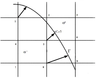
Definition: a grid point is called regular if all the grid points in the centered 5-point

stencil are on the same side of the interface; otherwise, a grid point is called irregular if not

all the grid points in the centered 5-point stencil are on the same side of the interface.

For example, in Figure 3.1, point 3, 4, 7 are regular grid points, while point

28

Figure 3.2 Interface, Regular and Irregular Points.

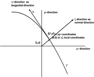
We consider a fixed point (x*,y*) on the interface, and define a local ξ-η coordinate

system by

  

− + −

− =

− + −

=

. cos *) (

sin *) (

, sin *) (

cos *) (

θ θ

η

θ θ

ξ

y y x

x

y y x

x

(3.4)

where θ is the angle between the x-axis and the normal direction, pointing to the direction of

a specified side, say the “+” side. At the point (x*, y*), the interface Γ can be written as

0 ) 0 ( ' , 0 ) 0 ( )

( _{= =}

=χ η χ χ

ξ with . (3.5)

29

Figure 3.3 An Irregular Grid Point, its Orthogonal Projection, and the Local Coordination.

Note that under the local coordinate transformation (3.4), the partial differential

equation (3.1) remains unchanged, that is:

] [ ]

[uξξ +uηη +ku = f . (3.1a)

3.3 Interface Relations

Let (x*, y*) be a point on the interface Γ. Assume that u(x,y) has second order

derivative in the neighborhood of (x*, y*) corresponding to the local coordinates at (0, 0).

Then from jump condition (3.2), we can immediately have

w u

30

Since (3.5), we can use the notation [u] = w(η) and [un] = g(η) in local coordinate

system. Differentiating (3.2) with respect to ξ along the interface, we get

g u

uξ+ = ξ− + . (3.7)

Differentiating (3.2) with respect to η along the interface, we get

) ( ' ] [ ' ]

[uξ χ+ uη =w η . (3.8)

Setting η=0, we get

'

w u

u+ ₌ − ₊

η

η . (3.9)

Differentiating (3.8), we obtain

) ( '' ] [ ' ] [ ] [ ' '' ] [ χ η η χ χ _{ξ ξη ηη}

ξ u u u w

d d

u _{+ + + = .}

Setting η=0, we get

'' '' )

(u u w

u

u+ ₌ − ₊ − ₋ + _{χ +}

ξ ξ ηη

ηη . (3.10)

In local coordinates, (3.3) can also be written as

2 ) ' ( 1 ' ' χ χ χ _{ξ η} η ξ − = − + + − − + + g u u u

u . (3.11)

Differentiating (3.11) with respect to η along with the interface, we have

). ) ' ( 1 '' ' ) ( ) ' ( 1 )( ( ' '' ' ) ( ' '' ' ) ( ' 2 2 χ χ χ η χ η χ χ η χ χ χ η χ _{ξη η η ξξ ξη η η} ξξ + + + + − − + = − − + + + + − − − − + g g u u d d u u u u d d u u (3.12)

Setting η=0, we get

' ''

)

(u u u g

u u

uξη+ = ξ−− ξ+ + η+ − η− χ + ξη− + . (3.13)

31 − + − + − − + + − = − + − −

+u u u ku ku f f

u_{ξξ ηη ξξ ηη} .

Solving for uξξ+, then

] [f kw u u u

uξξ+ = ξξ− + ηη− − ηη+ − + . (3.14)

These interface relation are used in deriving the finite difference method in later

section discussing correction term.

3.4 The Finite Difference Scheme of the IIM

At regular grid points (xi, yj), we can use the standard central five-point stencil finite

difference schemes . 2 ) , ( , 2 ) , ( , 1 , 1 , , , 1 , 1 y j i j i j i j i yy x j i j i j i j i xx h u u u y x u h u u u y x u − + ≈ − + ≈ − + − + (3.15)

If the solution is 2nd order continuous or higher, then it relatively easy to show that

the locate truncation error in these points are O(h2) in previous chapter.

We now focus on irregular grid points, which the solutions are discontinuous across

interface. Taking an irregular grid point (xi, yj), we try to develop the modified finite

difference scheme like following

ij ij ij k k j j i i

ku ku f C

s

k

k + = +

∑

= + + 1 ,

32

where the summation is take over ks neighborhood points center at (xi, yj), and γs are the

coefficients of the finite difference scheme. Our goal is to find proper coefficients γs and Cs,

such that the finite difference scheme is still second order accurate

Generally speaking, the wave number k is usually constant. And we would like

coefficient γs still keep as same as the ones in standard 5-point central finite difference

scheme. That is, the coefficients are γk =1/h2 for the four neighbors of (xi, yj), and −4/ h2 for

the master grid point (xi, yj).

3.5 Correction Terms at Irregular Grid Points

The Taylor expansion of u(xi+ik, yj+jk) about (xi, yj) under the local coordinates is

),

(

2

1

2

1

)

,

(

)

,

(

3 2

2

_u

_u

_u

_O

_h

u

u

u

u

y

x

u

k k

k k

k k

j j i

i _{k k}

+

+

+

+

+

+

=

=

± ±

±

± ±

± +

+

ηη ξη

ξξ

η ξ

η

η

ξ

ξ

η

ξ

η

ξ

(3.17)

where the “+” or “−” sign is chosen depending on whether (ξk, ηk) lies on the “+” or “−”

side of interface Γ. After the expansions of all terms, u(xi+ik, yj+jk), used in the finite

difference equation (3.16), the local truncation error Tij can be espressed as a linear

33

).

(

|}

max{|

)

,

(

)

,

(

)

,

(

3 12 11 10 9 8 7 6 5 4 3 2 1 1

h

O

C

f

ku

u

a

u

a

u

a

u

a

u

a

u

a

u

a

u

a

u

a

u

a

u

a

u

a

C

y

x

f

y

x

ku

y

x

u

T

k ij ij j i j i k k j j i i k ij s k k

γ

γ

ξη ξη ηη ηη ξξ ξξ η η ξ ξ

+

−

−

−

+

+

+

+

+

+

+

+

+

+

+

=

−

−

−

=

− − + − + − + − + − + − + − = + +

∑

(3.18)

The quantities f± are the limiting values of the function f at (xi*, yj*) from the “+” or “−” side

of the interface. The coefficients {aj} depend only on the position of the stencil relative to the

interface. They are independent of the PDE, u, k, f and the jump conditions w and g. If we

define the index set K+ and K− by

} " " ) , ( : { _{± Γ} =

± _{k is on the side of}

K ξ_k η_k .

Then the {aj}’s are given by

. , , , 2 1 , 2 1 , 2 1 , , , , , , 12 11 2 10 2 9 2 8 2 7 6 5 4 3 2 1

∑

∑

∑

∑

∑

∑

∑

∑

∑

∑

∑

∑

+ − + − + − + − + − + − ∈ ∈ ∈ ∈ ∈ ∈ ∈ ∈ ∈ ∈ ∈ ∈ = = = = = = = = = = = = K k k k k K k k k k K k k k K k k k K k k k K k k k K k k k K k k k K k k k K k k k K k k K k k a a a a a a a a a a a a γ η ξ γ η ξ γ η γ η γ ξ γ ξ γ η γ η γ ξ γ ξ γ γ (3.19)

Using the interface relations from (3.6) to (3.14), we can eliminate the quantities from

one side, say “+” side, using the quantities from the other side, say “−” side, and combining

34 ), ( |} max{| ) ( ) ( ) 1 ( ) 1 ( ) ( ) ( ) ( 3 12 11 10 9 8 7 6 5 4 3 2 1 h O C T f ku u a a u a a u a a u a a u a a u a a T k ij ij ij γ ξη ηη ξξ η ξ + − + − − + + − + + − + + + + + + + = ∧ − − − − − − − − (3.20) where ). '' ] ([ ) '' '' ( '' ' ) '' ( ' 8 10 8 4 10 12 6 12 2 w kw f a g a a a w a w a a g a w a T_ij − + + − + + + + + + = ∧ χ χ χ _(3.21)

Luckily, if we choose the coefficients γs as for standard 5-point central finite

difference scheme, then following equations are satisfied

. 0 , 1 , 1 , 0 , 0 , 0 12 11 10 9 8 7 6 5 4 3 2 1 = + = + = + = + = + = + a a a a a a a a a a a a (3.22)

In addition, let

), '' ] ([ ) '' '' ( '' ' ) '' ( ' 8 10 8 4 10 12 6 12 2 w kw f a g a a a w a w a a g a w a T C_{ij ij}

− + + − + + + + + + = = ∧ χ χ χ (3.23)

here, Cij depends on the curvature (w’’) of the interface, which means it is difficult to get an

analytic expression for the correction terms.

Thus, we have a method that the local truncation error at (xi*, yj*) in (3.18) is second

order convergence guaranteed in theory. Later in our numerical experiments results, the

35

Since the standard 5-point central finite difference scheme is used, and only the

right-hand sides of the finite difference equations need to be modifies by adding a correction term.

So the Fast Fourier Transformation solver as we described in previous chapter can be applied

to solve the system of finite difference equations. This makes the Immersed Interface Method

very efficient because the computational cost on the irregular points is relatively small.

Further in next chapter, under the augmented strategy, this IIM method still can be used

36

CHAPTER 4

Augmented Strategies

In many interface problems, the jump conditions for the solution U and the derivative

of the solution Un in the interface are coupled together, and one of them are usually unknown.

We start with assume the unknown jump condition as some augmented variable g of

codimension, and its discrete form G. The approximate solution U and the augmented

variable G together form a large linear system representing the original problem, thus it was

relatively easy to be understood but sometime too big to solved. Then, by eliminate U from

the matrix vector equations, we try to solve for the augmented variable G using the Schur

complement system, which is generally much smaller than that for U. GMRES iterative

method is used first solving the original problem, with assumed initial augmented variable;

then finding the residual of the constraint using the computed approximate solution given the

augmented variable.

Augmented method do not required a Green’s function, and no need to set up the

system of equations; and it can be applied to general PDEs with or without source term. All

boundary conditions shall be working just fine. Only high precision data type required when

implementation Schur complement. The only way to derive an accurate algorithm in that

kind of problem is perhaps the augmented approach.

The original idea of the augmented strategy for the interface problem is introduced in

[21] to solve elliptic interface problems, and then further developed in [22] applied to

37

4.1 The Augmented Variable

In this dissertation, we only studied Dirichlet boundary condition. Other boundary

condition such as Neumann and Robin, however, can be derived using same methodology.

Since Dirichlet boundary condition, we have already know the solution u at boundary,

u=w(x,y), (x,y)∈Γ. so it is natural to select the normal derivative [un] as the augmented

variable g. Further by discretization, we can write [u]Γ as W={W1, W2, … Wnb} and [un] Γ as

G={G1, G2, … Gnb}.

4.2 Discrete System of Equations in Matrix-Vector Form

From previous chapter, we knew that the correction term Cij depends on {Gk} and

{Wk} continuously. Then the Helmholtz equation (1.2) can be written as following discrete

from

F G W B

AU_{+ ( , )= , (4.5)}

where U and F are the vectors formed by {Uij} and {Fij}. From (3.23), we knew that B(W,G)

is a linear function of W and G, and can be written as

W B BG G W B

1

) ,

( _{= −} , (4.6)

where B and B1 are two matrices with entries. Thus (4.5) becomes

1

1W F

B F BG

38

On the other hand, if the solution U from the system (4.7) is known, we can

interpolate {Uij} linearly to get {U_n±(X_k)}, which is an approximation to the normal derivative

from each side of the interface at {Xk}, 1 ≤ k ≤ nb . The interpolation scheme is very

important to the accuracy of our augmented algorithm, we will discuss it in more detail next

section. Since the interpolation is linear, we can represent it as following

W DG

CU _{+ = , (4.8)}

where C and D are the linear interpolation scheme to approximate W.

Combining (4.7) and (4.8) together, we have

      =          

 

W F

G U

D C

B A

1 _{. (4.9)}

Remark: A, B, C and D represent the operation of their respect scheme, and they may not be

written explicitly into matrix format.

4.3 Least Squared Interpolation

In this study, we involved the complex number least squared interpolation scheme from a

Cartesian grid to form interface. It is almost identical to the work in real number [18]. The

performing of this least square interpolation scheme is crucial to the accuracy and the

iterations of the GMRES, and thus irreplaceable to whole augmented method.

39

∑

= + + − − = s k k k

k i i j j

k

n x y U C

U 1 , * * * * ) ,

( γ . (4.10)

where ks is the number of grid points involved in the interpolation scheme, ( xi*, yj*) is the

closest grid point to the projected interface point (x*, y*), C is the correction term and γk. is

the coefficients for the interpolation. Note that γk and C are depend on (x*, y*). It is clear that

we have to determine the coefficients {γk} and C to complete the interpolation.

The coefficients {γk} are determined by minimizing the interpolation error of (4.10)

when Ui*+ik, j*+jk is substituted with the exact solution u(xi*+ik, yj*+jk). Using the local

coordinates system    − + − − = − + − = . cos *) ( sin *) ( , sin *) ( cos *) ( θ θ η θ θ ξ y y x x y y x x (4.11)

Centered at the point (x*, y*), and denoted the local coordinates of (xi*+ik, yj*+jk) as (ξk, ηk),

we have the following from the Taylor expansion at (x*, y*) or (0,0) in the local coordinates:

). ( 2 1 2 1 ) , ( ) y , (x 3 2 2 +j * j +i

i* _{k k}

h O u u u u u u u u k k k k k k k k + + + + + + = = ± ± ± ± ± ± ηη ξη ξξ η ξ η ξ ξ η η ξ η ξ (4.12)

where the “+” or “-“ sign is chosen depending on whether (ξk, ηk) lies on the “+” or “-“ side

of the interface Γ, and u±, uξ±, …, uηη± are evaluated at local coordinates (0,0), or (x*,y*) in

the original coordinates system. Be careful with these two coordinate system, they are

confusing yet necessary for different computing function.

We carry out this expansion for all the grid points involved in the interpolation

40 combining likely terms and re-arrange them, we have

, *) *, ( 12 11 10 9 8 7 6 5 4 3 2 1 C u a u a u a u a u a u a u a u a u a u a u a u a y x U_n − + + + + + + + + + + + ≈ + − + − + − + − + − + − − ξη ξη ηη ηη ξξ ξξ η η ξ ξ (4.13)

where the {ai} are defined as following

. , , , 2 1 , 2 1 , 2 1 , , , , , , 12 11 2 10 2 9 2 8 2 7 6 5 4 3 2 1

∑

∑

∑

∑

∑

∑

∑

∑

∑

∑

∑

∑

+ − + − + − + − + − + − ∈ ∈ ∈ ∈ ∈ ∈ ∈ ∈ ∈ ∈ ∈ ∈ = = = = = = = = = = = = K k k k k K k k k k K k k k K k k k K k k k K k k k K k k k K k k k K k k k K k k k K k k K k k a a a a a a a a a a a a γ η ξ γ η ξ γ η γ η γ ξ γ ξ γ η γ η γ ξ γ ξ γ γ (4.14)

Since u+_=u-_{+w and u}

n+=un-+g. and the interface relations. We can express all the quantities

from the “+” side in (4.13) in terms of those from the “-“ side and the known quantities.

Thus , when Ui*+ik, j*+jk is substituted for the exact solution u(xi*+ik, yj*+jk) , (4.10) can be

written as . ] [ ] [ ] [ ] [ ] [ ] [ ) ( ) ( ) ( ) ( ) ( ) ( ) , ( ) , ( 12 10 8 6 4 2 12 11 10 9 8 7 6 5 4 3 2 1 12 11 10 9 8 7 6 5 4 3 2 1 1 * * * * C u a u a u a u a u a u a u a a u a a u a a u a a u a a u a a C u a u a u a u a u a u a u a u a u a u a u a u a C y x u y x U s k k k k j j i i k n − + + + + + + + + + + + + + + + + + + = − + + + + + + + + + + + = − = − − − − − − + − + − + − + − + − + − = + + −

_∑

ηη ξη ξξ η ξ ξη ηη ξξ η ξ ξη ξη ηη ηη ξξ ξξ η η ξ ξ γ

To minimize the interpolation error, we should set the following linear system of equations

41 . 0 , 0 , 0 , 0 , 1 , 0 12 11 10 9 8 7 4 3 4 3 2 1 = + = + = + = + = + = + a a a a a a a a a a a a (4.15)

If the linear system (4.15) has a solution, then we can obtain a second-order interpolation

scheme for the normal derivative un- by choose an appropriate correction term C. From (4.12)

and (4.15), we can see that the system of equations for the {γk} is independent of the jump

conditions which means we can calculate {γk} outside of GMRES iteration.

In this study, we choose between 6 to 16 closest grid points to (x*,y*) as the

interpolation stencil. If less than 6 different grid points (ks > 6) in a neighborhood of (x*,y*)

are used in the interpolation, we will have an under-determined system of linear equation

system. If more than 16 points are chosen, then the computing cost will be very high without

significant accuracy improvement.

We chose SVD method to solve (4.15). The SVD algorithm is very stable and can be

found in many software packages, such as Linpack and Lapack. The SVD solution has the

smallest 2-norm among all feasible solutions

} ) ( { min ) ( 1 2 1 2 *

∑

∑

= = = s k s k k k k k k γ γ γ .

For such a solution, the magnitude of γk* is well under control, which in important to the

stability of the entire algorithm. Once the {γk}’s are computed, then the {ak}’s can be

obtained quickly. Now the correction term C is determined from following:

). ' ' ' ' ( ) ' ' ' ' ( ]) [ ' ' ' ' ( ' 12 10 8 6 4 2 g w a g w a f w g a w a g a w a C + + − + + − + + + = χ χ χ (4.16)

42 g C U

y x U

s

k k

k

k

j j i i k

n ≅

∑

− +

=

+ + +

1

* , *

*) *,

( γ . (4.17)

In this study, the interface is represented by the zero set of a level set function, the

least squares interpolation is used to approximate the surface derivatives using their values at

the orthogonal projections of irregular grid points. The accurate with local support is

second-order. It is robust in smooth error distribution. The trade-off is that we have to solve a an

underdetermined 6× ks linear system of equations (ks ≥ 6), which is manageable.

4.4 Schur complement system

It is possible to directly solve the linear equation system in (4.9). However, by doing so, we

have to deal with a matrix of O((m × n × nb )2). This is way too much computing cost without

an existing fast solver. The more efficient way is to using Schur complement and GMRES

method, which we can also take advantage of new FFT passion solver we discussed in

previous chapter.

By solving for U from (4.7), then substitute it back into (4.8), we can eliminating U

from (4.9), and now have another much smaller O((nb)2) linear system

1 1 1 ₎

(D CA− B G W CA− F

− =

− , (4.18)

on the left hand side of the equation, D-CA-1B is the Schur complement of A. If the least

square interpolation C is second order approximation to the continuous jump condition on the