Multi-Sensor Calibration and Validation of the UWO-PCL Water Vapour Lidar

(1)

Western University Western University

Scholarship@Western

Electronic Thesis and Dissertation Repository

12-11-2012 12:00 AM

Multi-Sensor Calibration and Validation of the UWO-PCL Water

Vapour Lidar

Robin Wing

The University of Western Ontario Supervisor

Dr. R.J. Sica

The University of Western Ontario Graduate Program in Physics

A thesis submitted in partial fulfillment of the requirements for the degree in Master of Science © Robin Wing 2012

Follow this and additional works at: https://ir.lib.uwo.ca/etd

Part of the Atmospheric Sciences Commons, Climate Commons, and the Optics Commons

Recommended Citation Recommended Citation

Wing, Robin, "Multi-Sensor Calibration and Validation of the UWO-PCL Water Vapour Lidar" (2012). Electronic Thesis and Dissertation Repository. 981.

https://ir.lib.uwo.ca/etd/981

This Dissertation/Thesis is brought to you for free and open access by Scholarship@Western. It has been accepted for inclusion in Electronic Thesis and Dissertation Repository by an authorized administrator of

(2)

MULTI-SENSOR CALIBRATION AND VALIDATION OF THE UWO-PCL

WATER VAPOUR LIDAR

(Spine title: Calibration of the PCL Water Vapour Lidar)

(Thesis format: Monograph)

by

Robin Wing

Graduate Program in Physics and Astronomy

A thesis submitted in partial fulfillment

of the requirements for the degree of

Masters of Science

The School of Graduate and Postdoctoral Studies

The University of Western Ontario

London, Ontario, Canada

c

(3)

THE UNIVERSITY OF WESTERN ONTARIO

School of Graduate and Postdoctoral Studies

CERTIFICATE OF EXAMINATION

Supervisor:

. . . . Dr. R. J. Sica

Supervisory Committee:

. . . . Dr. P. G. Brown

. . . . Dr. M. Zinke-Allmang

Examiners:

. . . . Dr. M. Houde

. . . . Dr. P. Barmby

. . . . Dr. J. Voogt

The thesis by

Robin Wing

entitled:

Multi-sensor Calibration and Validation of the UWO-PCL Water Vapour Lidar

is accepted in partial fulfillment of the requirements for the degree of

Masters of Science

. . . . Date

. . . .

Chair of the Thesis Examination Board

(4)

Acknowlegements

I would like to thank Dr. R.J. Sica for his support, guidance and understanding over the past few years. I truely appreciate the experiences I have had and the lessons I have learned while working in the PCL lab. I would also like to thank Dr. P.S. Argall for his support in the lab and Dr. D.N. Whiteman for organising the PCL water vapour calibration campaign. I would like to acknowledge the tremendous support I have recieved from the departmental staff; my advisory committee members, Dr. P.G. Brown and Dr. M. Zinke-Allmang; B. Stonehouse at UWO Facilities Management; P. Duenk and C. Rasenberg at the Environmental Science Western Field Station; the NASA campaign team; and all the workstudy students who have helped our lab to record hundereds of hours of observations. Finally, I would like to thank my group members, past and present, E. McCullough, B. Iserhienrhien, F. Olofsson, J. Khanna, J. Bandoro, P. Argall, and A. Jalali.

(5)

Abstract

The Purple Crow Lidar (PCL) has recently participated in a water vapour validation cam-paign with the NASA/GSFC Atmospheric Laboratory for Validation/Interagency Collaboration and Education (ALVICE) Lidar. The purpose of this calibration campaign is to ensure that PCL water vapour measurements are of sufficient quality for use in scientific investigations of atmo-spheric change and to be included in the Network for the Detection of Atmoatmo-spheric Climate Change (NDACC) data base. The detection of long term changes in water vapour concen-tration, particularly in the upper troposphere and lower stratosphere (UTLS), is an issue of pressing scientific, ecological and societal concern.

The field campaign took place at the University of Western Ontario Environmental Re-search Field Station near London Ontario Canada, from May 23rd to June 10th 2012 and resulted in 57 hours of measurements taken over 12 clear nights. On each night a minimum of one RS92 radiosonde was launched. In addition, 3 cryogenic frost-point hygrometer (CFH) sondes were launched on clear nights over the course of the campaign. Measurements were obtained from near the surface up to∼20 km by both lidar systems, the radiosondes, and the CFH balloons. These measurements were used to calibrate profiles of water vapour mixing ratio by the newly relocated PCL.

Comparisons between measurements of water vapour mass mixing ratio taken by RS92 ra-diosondes, Cryogenic Frostpoint Hygometers, and the ALVICE and PCL lidars has resulted in the derivation of a system calibration factor ofξsys=0.7545. The application of this calibration

factor to PCL retrievals has allowed for the validation of PCL water vapour mass mixing ratio profiles to within±5% between the altitudes of 2 km and 9 km.

Keywords: Raman-scatter lidar, UTLS water vapour, multi-instrument calibration, ra-diosonde, crygenic frost point hygrometer

(6)

List of Figures

1.1 An atmospheric pressure profile calculated using the Barometric Formula. . . . 4

1.2 An atmospheric temperature profile based on the US Standard Atmosphere val-ues. [26] . . . 6

1.3 A phase transition diagram for water. . . 7

1.4 Enthalpy of fusion and vapourization of water. [61] . . . 9

1.5 Atmospheric absorption bands for water. [24] . . . 10

1.6 Infinite pool of water below a vacuum. [59] . . . 13

1.7 Stokes and anti-Stokes shifts with respect to Rayleigh scatter. PCL water vapour measurements rely on Stokes, or red-shifted Raman scatter from 532 nm. . . 20

1.8 Energy transitions for vibrational and rotational Raman scattering. [3] . . . 21

1.9 Raman scatter showing the O-branch, Q-branch, and S-branch. . . 22

1.10 Water filter transmission at 293 K. [53] . . . 22

1.11 Water filter transmission at 213 K.[53] . . . 23

2.1 PCL schematic diagram containing Hg telescope and receiver system. . . 25

2.2 Schematic of the Litron LPY-7000 laser head. . . 26

2.3 Effect of doubler crystal temperature on laser output power. . . 28

2.4 Effect of room temperature on laser output power. . . 29

2.5 The output power of the laser can be modulated by varying the delay between triggering of the Oscillator (blue), Pre-amplifier (magenta), and Amplifier (yel-low). The time delay of the emitted pulse is shown in green. [31] . . . 31

2.6 Schematic of beam expander. [60] . . . 33

2.7 Depiction of far field divergence from a laser aperture or terminal optic. . . 34

2.8 Original blueprint for the PCL optical transmission path. . . 35

2.9 Confirming the focal length of the liquid mercury telescope is 5.175 m. The red line represents measurements of the height in meters above the surface of the mirror. The blue curve is a fit to the count rates measured by the detector system while the mirror is rotating slowly. The green points are the count rates measured by the detector system while the mirror is rotating quickly. The mirror is unstable between the blue and green curves. . . 37

2.10 Schematic of the liquid mercury telescope from Borra et al. (1992). [8] . . . 37

(10)

2.11 A plot which describes the leveling of the surface of the telescope dish. Green squares represent shims placed under the base of the mirror, red triangles rep-resent lead weights hung from the rim of the mirror, blue diamonds are mirror surface height measurements made from a mounted engineer’s clock. The mir-ror is leveled to better than 1:5000. . . 40 2.12 A schematic of the reworked PCL detector box. Adapted from [10] . . . 41

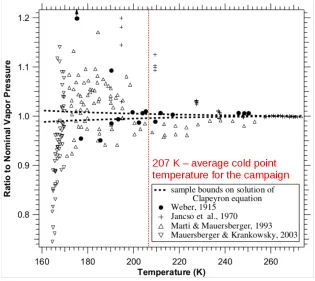
4.1 Experimental data measuring SVP over ice. Text in red indicates the average cold point temperature for the PCL calibration campaign. Taken and modified from Murphy and Koop 2005 [38] . . . 53 4.2 Model outputs measuring SVP over ice with respect to the Goff-Gratch

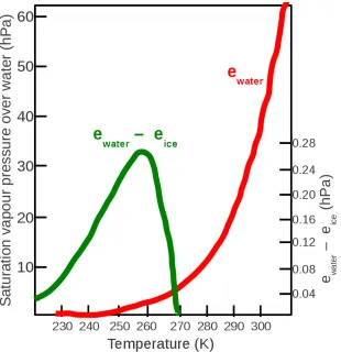
equa-tion. Taken and modified from Holger V¨omel [64] . . . 54 4.3 Variations in SVP with temperature over water (red) and between water and ice

(green). Adapted from [68] . . . 55 4.4 Variation between SVP models between 14 and 20 km for radiosonde data

taken May 24 at 3:39 UTC. There is a factor of approximately two between calculations of the SVP according to the Tsonis and Murphy-Koop models. . . 56 4.5 Ratios of SVP models for water and ice as a function of temperature. . . 56 4.6 Ratios of SVP models to Wexler 1976. . . 57 4.7 Percent difference of mass mixing ratios generated from Wexler minus

Murphy-Koop model outputs from RS92 data taken during the PCL calibration cam-paign. The Wexler model has a wet bias with respect to the Murphy-Koop model between 8 km and 14 km. . . 58 4.8 Uncertainty in RS92 temperature retrievals. Blue is measurement uncertainty,

black is uncertainty due to solar heating, and red is total uncertainty. [22] . . . . 59 4.9 Percentile difference profile between RS92 RH profiles and CFH RH profiles.

[35] . . . 60 4.10 Percent difference between Murphy-Koop 2005 and Tsonis 2002 at altitudes

from 275 m to 30 km. . . 61 4.11 Schematic of the cryogenic frost point hygrometer (CFH). Shown is the

cryo-gen tank which holds the carbon tetraflouride, the heater coil, the mirror, and the optical frost layer detection system Taken from [62] . . . 62 4.12 Initial CFH-lidar comparison contaminated by fluorescence. Taken from [28] . 63 4.13 CFH-lidar comparison up to 18 km . Taken from [33] . . . 64

5.1 The scale factor is only generated from measurements between 3 and 8 km. . . 67 5.2 Percent difference between each RS92 MMR profile and the hourly profile from

PCL. . . 69 5.3 Percent difference between the ensemble of RS92 and PCL profiles of MMR

with RMS errors. . . 69 5.4 Comparison of the percent difference plots between RS92&PCL and RS92&CFH.

[35] . . . 71 5.5 Percent difference with height for PCL and ALVICE MMR profiles. . . 72

(11)

5.6 Example of a scaled tropospheric PCL lidar profile compared to an RS92 pro-file and an ALVICE propro-file accompanied by a percent difference plot between

each of the CFH, RS92 and ALVICE with PCL. . . 73

5.7 Percent difference between the ensemble of ALVICE and PCL profiles of MMR with RMS errors. . . 73

5.8 PCL and ALVICE stratospheric water vapour returns. . . 74

5.9 Unexpected drop in CFH VMR compared to both lidars. . . 75

5.10 Unexplained deviations between the CFH and the lidars above 10.5 km. . . 75

5.11 Approximation for the flight path for the June 8th CFH. . . 76

5.12 Standard CFH and iMet plot for June 8th. CFH (purple), RS92 radiosonde (red), iMEt radiosonde (yellow), and SVP curve (black dots). 100% RH is occuring near 10 km. . . 78

5.13 PCL and ALVICE stratospheric water vapour returns. . . 79

6.1 Ground loop contaminating PCL returns below∼3 km. . . 81

A.1 PCL nightly colour plot of tropospheric water for May 24th. . . 92

A.2 PCL, ALVICE, and RS92 mass mixing ratio profiles for May 24th at 3:39 UTC. 92 A.3 PCL, ALVICE, RS92, and CFH mass mixing ratio profiles for May 24th at 6:59 UTC. . . 93

A.4 PCL and ALVICE volume mixing ratio profiles for May 24th at 3:39 UTC. . . . 93

A.5 PCL, ALVICE, and CFH volume mixing ratio profiles for May 24th at 6:59 UTC. 94 A.6 RS92 profiles for temperature (red) and RH (black) on May 24th at 3:39 UTC. . 94

A.7 RS92 profiles for temperature (red) and RH (black) on May 24th at 6:59 UTC. . 94

A.8 CFH profile for temperature on May 24th at 4:02 UTC. . . 95

A.10 PCL,ALVICE, and RS92 mass mixing ratio profiles for May 25th at 3:57 UTC. 96 A.11 PCL and ALVICE volume mixing ratio profiles for May 25th at 3:57 UTC. . . . 97

A.25 PCL nightly colour plot of tropospheric water for June 4th. . . 104

A.26 PCL,ALVICE, and RS92 mass mixing ratio profiles for June 4th at 3:22 UTC. . 104

A.27 PCL,ALVICE, and RS92 mass mixing ratio profiles for June 4th at 5:40 UTC. . 105

A.28 PCL and ALVICE volume mixing ratio profiles for June 4th at 3:22 UTC. . . . 105

(12)

A.29 PCL and ALVICE volume mixing ratio profiles for June 4th at 5:40 UTC. . . . 105 A.30 RS92 profiles for temperature (red) and RH (black) on June 4th at 3:22 UTC. . 106 A.31 RS92 profiles for temperature (red) and RH (black) on June 4th at 5:40 UTC. . 106 A.32 PCL nightly colour plot of tropospheric water for June 6th. . . 107 A.33 PCL,ALVICE, and RS92 mass mixing ratio profiles for June 6th at 3:12 UTC. . 107 A.34 PCL,ALVICE, and RS92 mass mixing ratio profiles for June 6th at 5:29 UTC. . 108 A.35 PCL and ALVICE volume mixing ratio profiles for June 6th at 3:12 UTC. . . . 108 A.36 PCL and ALVICE volume mixing ratio profiles for June 6th at 5:29 UTC. . . . 109 A.37 RS92 profiles for temperature (red) and RH (black) on June 6th at 3:11 UTC. . 109 A.38 RS92 profiles for temperature (red) and RH (black) on June 6th at 5:29 UTC. . 109 A.39 PCL nightly colour plot of tropospheric water for June 7th. . . 110 A.40 PCL and RS92 mass mixing ratio profiles for June 7th at 3:45 UTC. . . 110 A.41 PCL volume mixing ratio profiles for June 6th at 3:45 UTC. . . 111 A.42 RS92 profiles for temperature (red) and RH (black) on June 7th at 3:45 UTC. . 111 A.43 PCL nightly colour plot of tropospheric water for June 8th. . . 112 A.44 PCL,ALVICE, and RS92 mass mixing ratio profiles for June 8th at 3:53 UTC. . 112 A.45 PCL,ALVICE, RS92, and CFH mass mixing ratio profiles for June 8th at 6:51

UTC. . . 113 A.46 PCL, ALVICE, and CFH volume mixing ratio profiles for June 8th at 3:53 UTC. 113 A.47 PCL and ALVICE volume mixing ratio profiles for June 8th at 6:51 UTC. . . . 114 A.48 RS92 profiles for temperature (red) and RH (black) on June 8th at 3:53 UTC. . 114 A.49 RS92 profiles for temperature (red) and RH (black) on June 8th at 6:51 UTC. . 114 A.50 CFH profile for temperature on June 8th at 2:51 UTC. . . 115 A.51 PCL nightly colour plot of tropospheric water for June 10th. . . 116 A.52 PCL,ALVICE, and RS92, mass mixing ratio profiles for June 10th at 4:02 UTC. 116 A.53 PCL and ALVICE volume mixing ratio profiles for June 10th at 4:02 UTC. . . . 117 A.54 RS92 profiles for temperature (red) and RH (black) on June 10th at 4:02 UTC. . 117

(13)

List of Tables

1.1 Fractional concentration of gasses in Earth’s atmosphere. [68] . . . 4

2.1 Optical specifications for the liquid mercury telescope. . . 36

3.1 Water vapour mixing ratio equation atmospheric parameters. . . 45

3.2 Reflectivity of PCL detector box optics. . . 46

4.1 PCL-ALVICE field campaign log. . . 50

5.1 Table of derived lidar fitting factors and reduced chi-squared values for each night of good data during the campaign. . . 66

5.2 Table of the average percent difference between MMR values measured by PCL and ALVICE lidars for each night of good data during the campaign. Poor fits have percent differences greater than 10%, acceptable fits have differences between 5% and 10%, and excellent fits have differences less than 5%. . . 71

(14)

List of Appendices

Appendix A . . . 91 Appendix B . . . 118

(15)

Chapter 1 A Review of Some Atmospheric Concepts

1.1 Introduction

The atmosphere makes life on Earth possible. It shields us from harmful extplanetary

ra-diation; it moderates the surface temperature of the planet and insulates us from the diurnal

solar cycle; it allows for a common, well mixed reservoir of gasses from which organisms can

cycle necessary chemical compounds; and it provides a medium for the long range transport

and circulation of water.

The presence of water vapour in the atmosphere is a very important, but imperfectly

un-derstood, variable in the global atmospheric radiation balance. It is expected that in the

tro-posphere water vapour acts as a greenhouse gas and warms the atmosphere by absorbing and

remitting long wave infrared radiation. As the temperature of the atmosphere warms, it is

ex-pected that an increase in the concentration of water vapour in the air will occur. This process

in turn will cause more heating and act as a positive feedback mechanism.

However, as the concentration of water molecules increases in the lower atmosphere, it is

expected that more clouds will be formed as more moist air is lifted and cooled. Clouds are a

key component in reflecting incoming solar rays, preventing higher frequency light from being

absorbed and re-emitted from the surface. If this effect is dominant, it would act to cool the

lower atmosphere, limiting water-driven heating, which in turn limits cloud formation. This

effect is known as cloud feedback and is a sensitive negative feedback loop parameter in most

(16)

2 Chapter1. A Review ofSomeAtmosphericConcepts

global climate models.

The above mechanisms are well understood and are a part of the many complexities in

attempting to make model forecasts of global atmospheric change. A more full description of

these phenomena can be found in the IPCC 2007 report [25]. One of the major issues with

properly incorporating the effects of increased water vapour in both the troposphere and the

lower stratosphere is the absence of a long term, reliable, well calibrated measurements [25].

Currently, water vapour mixing ratio can be measured by various kinds of satellites such as

the Atmospheric Chemistry Experiment (ACE), through measurements from humidity sensors

mounted on commercial and research aircraft, by dropsonde and radiosonde campaigns, and

by Raman Lidar techniques [36]. Each instrument type has observational strengths and

weak-nesses and lidar is a no exception. The lidar technique provides excellent spatial and temporal

resolution measurements of water vapour mixing ratio but has limited geographic coverage,

requires extensive expertise for construction, maintenance and operation, and requires

calibra-tion and routine checks on data consistency. This thesis will focus on the calibracalibra-tion of Raman

lidar measurements of water vapour in the upper troposphere and lower stratosphere (UTLS).

1.2 Atmosphere Pressure for an Isothermal Atmosphere

The homogeneous, neutral atmosphere is a relatively well mixed, stably stratified fluid

extend-ing from the planet’s surface to the turbopause, a region which is nominally located between

95 and 115 km in altitude. The gravitational attraction between Earth and its atmosphere gives

rise to an exponential decrease in pressure with height, as lower layers of gas are compressed

under the weight of layers at higher altitudes. By invoking the equation of state for an ideal gas,

(1.1) wherePis the gas pressure (Pa),ρis the gas density in _mkg3,Ris the universal gas constant

(17)

1.3. AtmosphericComposition 3

which balances the pressure gradient force with gravity can be derived.

P= ρRT (1.1)

This condition, known as the Hydrostatic Equilibrium Equation, (1.2),

dP

dz +ρg=0 (1.2)

where g(z) is the gravitational acceleration and the surface value is 9.80665 _sm2, allows us to

characterize ane-folding height for the density curve of the atmosphere (1.4), wherekis

Boltz-mann’s Constant 1.3806488×1023 J_K, andMis the molar mass of air, which can be calculated

from a periodic table, is 0.0289644 _molkg. A typical value of the e-folding, or scale height, in

the region of Earth’s atmosphere is approximately 8 km. A curve representing this exponential

drop in pressure with altitude can be calculated using the Barometric Formula(1.3),

P= P0·exp

"

−g· M·z R·T0

#

(1.3)

whereT0 andP0 are the respective temperatures and pressures at the surface, and can be seen

in Figure 1.1.

H = kT

Mg(z) (1.4)

1.3 Atmospheric Composition

Within this well mixed region, the composition of the atmosphere is uniform. Table 1.1 details

the fractional concentration by volume for the most abundant gasses in Earth’s atmosphere.

Taken together, molecular nitrogen and molecular oxygen compose approximately 99.03% of

the air with the trace gasses comprising the remaining fraction of a percent in the dry

(18)

Figure 1.1: An atmospheric pressure profile calculated using the Barometric Formula.

Constituent Molecular Weight Fractional Concentration by Volume

Nitrogen (N2) 28.013 78.08%

Oxygen (O2) 32.000 20.95%

Argon (Ar) 39.95 0.93%

Water Vapour (H2O) 18.02 0-5%

Carbon dioxide (CO2) 44.01 380 ppm

Neon (Ne) 20.18 18 ppm

Helium (He) 4.00 5 ppm

Methane (CH4) 16.04 1.75 ppm

Krypton (Kr) 83.80 1 ppm

Hydrogen (H2) 2.02 0.5 ppm

Nitrous oxide (N2O) 56.03 0.3 ppm

Ozone (O3) 48.00 0-0.1 ppm

(19)

1.4. TemperatureStructure 5

values possible and is extremely variable in both space and time. This uncertainty in the

con-centration of water vapour can be intuitively to understood as the variation in the humidity of

our environment with temperature changes. The summer air is hot and humid, while the winter

air tends to be cold and dry. A more formal exploration of how moisture in the atmosphere

cycles and which physical parameters are important in its description are presented later in the

chapter.

1.4 Temperature Structure

Temperature variations are important parameters in characterizing and understanding the

at-mosphere. The atmosphere can be divided into four regions, each of which is marked by a

temperature gradient which is calculated from the hydrostatic balance equation (1.2) and a

for-mulation of the first law of thermodynamics (1.5) whereUis the internal energy of the system,

δQis an infinitesimal amount of heat supplied to the system by its surroundings, anddV is a

change in the volume of the system. The four regions of the atmosphere are the troposphere,

stratosphere, mesosphere, and thermosphere. For the purposes of this work only the lowest two

regions will be considered; the dynamicas and chemistry of water vapour in the mesosphere

and thermosphere will be ignored.

dU = δQ−PdV (1.5)

1.5 Troposphere

The troposphere is the lowest region extending from the surface of the planet up to nominally

10 km altitude and it is characterized by a negative lapse rate, convective and turbulent mixing,

(20)

Figure 1.2: An atmospheric temperature profile based on the US Standard Atmosphere values. [26]

our day-to-day weather phenomena. Using an appropriate value for the specific heat capacity

at constant pressure,cp=29.07_molJ_·_K, and the assumption of an adiabatically rising parcel of air

we can derive equation (1.6) the Dry Adiabatic Lapse Rate (DALR) which is equal to 9.8 _kmK.

Γd =−dT

dz =

g cp

≈9.8 K

km (1.6)

Given that water is a condensable gas and has easily accessible liquid, solid, and vapour states

over a normal range of atmospheric pressures, the contributions of water to the thermodynamics

of the atmosphere must be considered. Figure 1.3, shows the phase transition curves for water

and have been sketched based on values listed in the CRC [30].

As water evaporates and condenses in Earth’s atmosphere there is a flux of enthalpy into the

surrounding air. If we assume that the atmosphere is completely saturated with water vapour,

then the DALR must be modified to accommodate the enthalpy associated with the water which

results in a Moist Adiabatic Lapse Rate (MALR). The MALR is typically around 5 _kmK and is

given by (1.7)

Γm = g

cp          

1+ Lqs

RT

1+ 0.62L2qs

cpRH₂OT2           (1.7)

(21)

1.5. Troposphere 7

Figure 1.3: A phase transition diagram for water.

mixing ratio which will be defined later. The MALR is derived in a similar fashion to the

DALR accounting for the enthalpy of the water contained in the air [20].

As can be seen from (1.6) and (1.7) the presence of water vapour in the atmosphere plays a

crucial role in the temperature profile. If we imagine a parcel of dry air, composed of molecular

nitrogen and molecular oxygen, having an average molar mass of approximately 29 _molg [30]

then we know that by adding moisture to the air parcel we make it lighter as the molar mass of

water approximately 18 _molg [30]. Using the ideal gas law equation (1.1) we can see that the gas

constant for dry air, R, needs to be slightly altered to RH2O, taking into account the moisture

contained within the air parcel.

Above the troposphere is an intermediate region known as the tropopause. The tropopause

is a region where the lapse rate fluctuates about zero and can be thought of as an isotherm.

(22)

in atmospheric temperature. Values colder than 210 K are not uncommon. The significance

of this region of the atmosphere is that it acts as a partial barrier to the convective mixing of

moist, tropospheric air and the drier non-convecting stratosphere directly above it. However,

the transport of air across this region, known as stratosphere-troposphere exchange, can be

driven by localized and transient dynamical, chemical and radiative coupling processes [21].

These processes are essential for the water vapour inventory of the stratosphere [42].

1.6 Stratosphere

The stratosphere is the region directly above the tropopause and extends to roughly 50 km

altitude. The region gets its name from the stably stratified nature of the temperature profile.

Whereas the troposphere features a negative lapse rate, the stratospheric temperature profile

increases with increasing altitude due to the presence of ozone. This temperature inversion

suppresses convection and damps out the vertical motions of injected tropospheric air. The

ozone molecule, O3, absorbs incoming ultraviolet solar radiation and redistributes a portion of

the energy as increased temperature.

Accurately measuring stratospheric water vapour is of particular interest to climate

scien-tists as existing global climate models do not simulate temperature trends in the lower

strato-sphere very accurately and stratospheric chemistry-climate models cannot produce temperature

profiles which match observations [23]. Well calibrated measurements of stratospheric water

vapour are essential for calculating the radiative forcing on the stratosphere and for integration

into prognostic climate models.

1.7 Water Vapour in the Atmosphere

As was discussed in section 1.3, water vapour is a very important, poorly understood and

highly variable chemical species in the atmosphere. Its most critical role is manifested as a

(23)

1.7. WaterVapour in theAtmosphere 9

the planet’s atmospheric energy balance.

The following subsection will lay out a few qualitative points, summarized from [46],

ex-plaining why water vapour is such a potent atmospheric constituent and why it requires study.

Following the qualitative summary a few useful metrics for the quantization of water vapour

and saturation vapour pressure equations will be derived. Both of these ideas are of central

importance to the calibration effort in this thesis.

1.7.1 Qualitative Discussion

Water vapour has a very large ’latent heat’, hereafter properly referred to as enthalpy, associated

with all of its phase transitions. Figure 1.4 gives an indication of the magnitudes of these

enthalpies for the processes of vapourization and fusion [12]. As a result, the vapour pressure

of water, at equilibrium, has a very strong dependence on temperature. The two most important

consequences of this close connection between temperature and the phase state of water are:

i)Water vapour abundance varies strongly with season, altitude, and latitude.

(24)

ii)The local abundance of water vapour may be perturbed by large scale atmospheric

cir-culation patterns and convection, drawing it into regions where it is out of equilibrium with the

temperature of the environment.

Due to the associated enthalpies associated with changes in state, water can act as a vector

for the transport of significant amounts of energy throughout the atmosphere. For example, as

water undergoes vapourization at the surface it requires energy and decreases the temperature

of its surroundings. When that water vapour is then lifted convectively to an altitude where

it becomes energetically favourable to condense, the water molecules release energy into their

new environment and precipitate out of solution. From start to finish, this example transports

heat from the surface aloft and greatly changes the radiative balance of the local atmosphere.

The H2O molecule has a very complex set of absorption bands as can be seen in Figure

1.5. These absorption bands are interspersed with windows which transmit easily through the

moist lower layers of the atmosphere. Looking at Figure 1.5 it can be seen that the light which

Figure 1.5: Atmospheric absorption bands for water. [24]

the Sun emits in the visible portion of the spectrum is weakly absorbed by water vapour, and

(25)

based on its black-body temperature, the IR radiation is strongly absorbed and re-emitted in

several absorption bands which are associated with water vapour. This ”trapping” of long wave,

outgoing radiation, is the basic idea behind the ”greenhouse effect”, thus making water vapour

a prominent greenhouse gas. Further, the concentration of this gas is closely linked to the long

term warming trend of the troposphere as water is known to participate in a positive feedback

loop where warmer temperatures promote a higher atmospheric water vapour concentration

[23].

When water vapour condenses to form clouds of liquid or ice particles its optical properties

also change. As can be observed, clouds are often opaque in the visible portion of the spectrum,

and where once solar radiation passed freely through the atmosphere to the Earth’s surface, now

is reflected or absorbed by cloud layers. The clouds reflect incoming visible light and lower the

planets albedo, or reflection coefficient. With less light reaching the surface the planet should

cool. As was mentioned in the introduction to this thesis, the fundamental question: Does

increasing Earth’s water vapour budget heat or cool the planet? is still open for exploration.

1.7.2 Quantitative Discussion

There are several common methods for quantifying the amount of water vapour in the

atmo-sphere. The most basic measure is absolute humidity which is simply the number or mass

density of water molecules over the number or mass density of molecules of ”dry air” within

a given volume. From the mass density we can express the ’partial pressure’ of water vapour

relative to the total pressure of the gas mixture. We can invoke a slightly modified form of the

ideal gas law, equation (1.1), and define a partial pressure for water vapour, e, where ρvapour

is the mass density of water vapour, Rvapour is the gas constant for water vapour, andT is the

temperature of the gas mixture [68].

(26)

Carrying forward with the ideas of partial pressure and vapour mass density, two more metrics

can be defined:

a. The humidity mixing ratio,w

b. The absolute humidity,r

w= ρvapour

ρdry

(1.9)

r= w

wsaturation

(1.10)

where ρdry is the mass density of dry air and wsaturation is the saturation vapour mixing ratio

which will be elaborated on in the next section [68]. Relating the mixing ratio,w, to the partial

pressure of water vapour,e, using equation (1.11)

w Rdry

Rvapour

e

P−e =0.622

e

P−e (1.11)

WherePis the total pressure of the gas andRdryis the gas constant for air. The last (and most

useful for this thesis) metric is called relative humidityRH and is properly defined in equation

(1.12) [68].

RH = w

ws = e

es

P−es

P−e (1.12)

Many texts and papers neglect the second half of the equation and approximateRH by _ee s.

One of the lessons learned from the MOHAVE campaign, which will be discussed in a later

chapter, is that the contribution of the P−es

P−e is essential when determining RH in very cold, dry

environments like the lower stratosphere [29]. RH is seen to depend on pressure, which is a

function of temperature, e, which was shown earlier to be a function of temperature, and on

es, the saturation vapour pressure, which will be discussed in the next section and is also a

(27)

1.7.3 Saturation Vapour Pressure as Applied to the Atmosphere

Saturation vapour pressure (SVP) is a nuanced concept and some time will be taken to lay out

a precise description. The framework for the following derivation comes from [5] but more

detailed expressions from [38], [70], and [65] will be inserted where required.

Imagine an infinitely large and infinitely deep, flat, pool of water at constant temperature,T

depicted in Figure 1.6. Above this pool there is only vacuum and we assume that any walls or

surfaces are infinitely far away. The speed of water molecules depends upon the temperature of

the liquid. There should be an expectation speed for the molecules,<v>, which is proportional

to the square root of temperature, and the distribution of the speeds from the expectation value

should follow the Boltzmann distribution in a liquid.

Figure 1.6: Infinite pool of water below a vacuum. [59]

(28)

over come the inter-molecular cohesion of the liquid it can escape into the vacuum. This

process is evaporation,E, and it is only dependant on the temperature of the liquid. Again, we

are assuming that our infinite pool is sufficiently large that the enthalpy of vapourization of the

escaped molecule does not lower the temperature of the liquid.

Now we have some water vapour above the pool and it has some mass density, mvapour,

temperature,Tvapour(does not need to be the same as the liquid), and a distribution of molecular

speeds about< vvapour >. We should expect some of the molecules in the vapour to have low

kinetic energies and to collide with the surface of the liquid. When this happens the molecule

may be seized by the cohesive forces and condensed,C, back into the liquid state. We should

also expect that the number of condensation events is some function of the temperature of the

vapour and the number of vaporized molecules. Equation (1.13) summarizes the preceding two

paragraphs.

With these ideas about total evaporation and condensation we can define a net flux of water

molecules between the liquid and gaseous states, equation (1.14). It is important to note that

Fnetis the quantity that our instruments measure, notFup.

d(mvapour)

dt = E(Tliquid)C(Tvapour,mvapour) (1.13)

Fnet = Fup−Fdown (1.14)

In the previous section we defined the absolute humidity, w, as a vapour density ratio.

Fluxes are really just the rate of change in time of number densities. If we setTliquid =Tvapour =

Ttotalwe should be able to use equation ([?]) to work out the saturation mixing ratio,ws.

Fup

Fdown

=w< v(T)> /ws <v(T)> (1.15)

E

C =

w ws

(1.16)

(29)

temper-1.7. WaterVapour in theAtmosphere 15

ature andRH; however, we have not given a functional form. SVP is a very difficult quantity

to determine. It is very difficult to accurately measure the fluxes associated with an infinite flat

pool as the introduction of an instrument or a surface alters the rate of condensation, especially

at low temperatures [32]. Modelling the SVP also involves difficulties [38]. However, we can

begin to sketch out the generalized form that an SVP model should take.

Begining with the Clausius-Clapeyron equation (1.17) as given in [70].

d(es)

dt =

L

T(V −i) (1.17)

where Lis the enthalpy of condensation or sublimation, V is the specific volume of the

satu-ration vapour pressure for water vapour, andi is the specific volume of the saturation vapour

pressure over ice.

Next we need an equation of state to describe the gasses being modelled. We will use

a modified version of the ideal gas law (1.18) where Z is a measured compressibility factor

instead of a mass or a density.

PV =ZRT (1.18)

Combining equation (1.1) into equation (1.17) and separating like terms we arrive at

Equa-tion 1.19.

dP

P =

L

ZRT2₍₁+ i

v)dT

(1.19)

Now we need to select a temperature range (and appropriately mapped pressure range)

over which the equation will be valid. This is limited by the range over which measurements

or models ofLare available.

Z P2

P1

dlnP=

Z T2

T1

dT L

ZRT2₁+ i

V

(30)

Until this point in the derivation we have not had to make any approximations or rely on

measurements or modelling. Unfortunately, we now need an expression for both the enthalpy

of ice,Lice, and the enthalpy of water,Lwater, which are accurate over the temperature range of

interest. Much like with the lab experiments for measuring the SVP curve directly,

experimen-tal measurements of the enthalpy curves, such as the work done by Marti and Mauersberger

(1993) [32], are technically challenging and do not produce sufficiently reliable results for our

work.

The other approach for determining enthalpies at low temperatures is to write series

ex-pansions of the enthalpy terms, fit the terms with a polynomial and then extrapolate to low

temperatures. Unfortunately, there are a multitude of models to choose from, all of which

suffer from the typical blights of truncation, rounding, choice of fitting function, order, etc.

with large variations existing between models by different authors. Murphy and Koop (2006)

[38] wrote a review paper of the most prominent SVP models and came to the conclusion that

there is very little basis for any of the models or measurements within the temperature regime

of interest for this thesis. In chapter 4 a comparison of model outputs will be shown and the

reasoning behind the choice of model choice for this work will be discussed.

1.8 Atmospheric Scattering

The scattering of light off particles in the atmosphere is an everyday phenomenon; we see

bright, clear blue skies, white, grey and black clouds, red sunsets and sunrises, and at times

many other shades of pink, purple and green. All these different picture-perfect moments can

be described in terms of photons scattering offof atoms, molecules and aerosols.

In general, there are three major types of scattering which can occur: Mie, Rayleigh, and

(31)

1.8. AtmosphericScattering 17

1.8.1 Mie Scattering

Mie scattering happens when light scatterers offa particle with a radius much larger than the

wavelength of the incident photon. Surface effects, shape, and refractive index are all

impor-tant quantities to know when working with this kind of scattering. Mie scattering is typically

associated with lidar studies of aerosols and for the purposes of this thesis I will not consider

it.

1.8.2 Rayleigh Scattering

Rayleigh scattering is elastic scattering of a photon offa scattering target. Rayleigh scattering

is a central technique employed by PCL so it is important to examine its postulates, PCL’s data

acquisition, and address any discrepancies between the two.

Rayleigh scattering has five assumptions:

i) The scatterer must be smaller in size than the wavelength of the incident photon. The

PCL transmits at 532 nm and we assume that the bulk atmospheric scatterers are molecular

nitrogen and molecular oxygen typical cross sections for these molecules are estimated at 300

pm and 292 pm respectively [30]. Rayleigh scattering is valid for the majority of atmospheric

constituents. Care must be taken when larger particles such as aerosols are present in the

atmospheric sample.

ii) The scatterer must not be ionized. Most molecules below the ionosphere, altitudes

greater than approximately 90 km, are non-ionized. This work takes place in the lower and

middle atmosphere so we are safe in using Rayleigh techniques.

iii) The scatterers must have an internal index of refraction near unity. This condition

is required to prevent large phase changes in the photon wave fronts as they move into the

scatterer and out again. These phase changes can be conceptualized by recalling the definition

of the absolute index of refraction equation (1.21), wherecis the speed of light, vis the wave

(32)

nc

v =

r µ

0µ0

(1.21)

The index of refraction for air is usually given asn=1.000293 [19]. However, it is

impor-tant to note that other atmospheric constituents, most imporimpor-tantly water vapour (n ≈ 1.33) do

not satisfy this criterion.

iv)The scatterers must be isotropic molecules which do not experience dipole oscillations

when interacting with a photon. Neither molecular nitrogen nor molecular oxygen satisfies this

criterion due to their diatomic structures. Fortunately, a correction for anisotropy was given

by Cabannes which separates out the elastic component of the signal from the inelastic side

lobes [49]. To be correct what PCL truly measures is called Rayleigh-Cabannes scattering as

it assumes a correction for molecular anisotropy.

v)The scatterers must not have resonant frequencies near the frequency of the incident

pho-ton. For example, when the laser frequency of a lidar transmitter approaches the absorption line

of an atmospheric constituent the scattering cross section is significantly enhanced [49]. This

resonant scattering phenomenon is what allows lidars to determine atmospheric temperature in

regions such as the sodium layer in the upper atmosphere.

When we consider a photon ’scattering’ off an atom or particle what we are actually

en-visioning is an absorption and re-emission process. Imagine a molecule of nitrogen; it has a

central nucleus and a cloud of electrons surrounding it. Each of these electrons has a defined

energy associated with it. When a photon interacts with one of the electrons associated with

the molecule it raises the energy level of the electron to a ’virtual state’. These virtual states are

unstable arrangements and the electron quickly decays back to a lower energy state and emits

a photon with the exact same wavelength at which it was stimulated.

It can be shown that the intensity of a scattered beam has both angular and wavelength

dependence [34]. If a given molecule has a scattering cross section given by equation (1.23),

(33)

per unit volume then we can define an expression equation (1.22) for the scattering intensity.

I(x)= I0e−σN x (1.22)

σ= 2k4

3πN2

1−n2 (1.23)

This form can approximately be expressed in terms of the scattering intensity of linearly

polar-ized light offa dielectric sphere as a function of scattering angle expressed in equation (1.24)

whereφis the scattering angle andE0is the magnitude of the incident electric field.

I(φ)≈ E₀29π20c

2N2λ4 sin 2φ (1.24)

1.8.3 Raman Scattering

In contrast to Rayleigh scattering, Raman scattering is an inelastic process where a ray of

monochromatic light scatters offa molecule at different wavelengths than the incident ray. This

frequency shifting of scattered light happens when energy is transferred between the incident

photon and the scatterer, in increments which are proportional to the quantized rotational and

vibrational energy levels of the atom or molecule. Said another way: the scattered photon

either gains energy from the interaction and shifts to a higher frequency, a process known as

Stokes shift, or the scattered photon loses energy from the interaction and shifts to a lower

frequency, a process known as anti-Stokes shift. Since our scattering targets of interest are

mostly diatomic molecules we expect that there will be energy shift due to both the vibrational

as well as rotational transitions. Figure 1.7 represents the Raman transitions with respect to the

virtual state and the energy of the incident photon.

To characterize the possible energy states it is best to introduce two quantum numbers J

andv. Beginning with the idea of Bohrs atom we imagine electron shells which have discrete

energy levels. Combining two atoms together the allowable energy states become more

(34)

Figure 1.7: Stokes and anti-Stokes shifts with respect to Rayleigh scatter. PCL water vapour measurements rely on Stokes, or red-shifted Raman scatter from 532 nm.

sub-levels, v. For our purposes we will only allow∆J = 0,±2 and∆v = 0, ±1 which are the

allowable states of a diatomic molecule. A plot of three different Raman vibrational modes

with their attendant rotational wings is shown in Figure 1.8.

For a given Raman spectrum we can define a centralQ-branch transition where∆J =0 and

∆v= ±1. This spectral mode is associated with ”pure” vibrational scattering and is analogous

to the central Cabannnes line discussed in the previous section on Rayleigh scattering. When

∆J = +2 and v = 0 we enter a rotational side lobe known as the S-branch. The S-branch is

the ’blue-shifted’ or anti-Stokes wing of the spectrum. When∆J = −2 andv = 0 we enter

the other rotational side lobe known as the O-branch also known as the ’red-shifted’ or Stokes

wing of the spectrum. Figure 1.9 shows a diagram of this nomenclature scheme.

It is important to specify that PCL only seeks to make measurements of the Q-branch of

a Raman spectrum as these are pure vibrational lines. However, it is not possible to measure

an infinitely thin spectral width. Therefore, PCL also measures the O- and S- branches of

the desired spectra. Theoretically, this poses a problem as there is a temperature dependent

(35)

Figure 1.8: Energy transitions for vibrational and rotational Raman scattering. [3]

concluded that for the 1.11 nm filter in front of the PCL water channel there is a less than 5%

variation over the temperature range of 293 K to 213 K. His results are shown in Figures 1.10

and 1.11.

In Figures 1.10 and 1.11 the dashed line represents the filter bandwidth while the Raman

spectrum intensity is shown for two temperatures. At 293 K the filter fits the spectrum well

and there is minimal loss. At 213 K the sum of the product of the spectrum intensity and

transmission index is lower, indicating a poorer fit. Marcos Algara-Siller derived and applied

(36)

Figure 1.9: Raman scatter showing the O-branch, Q-branch, and S-branch.

(37)

(38)

Chapter 2 Lidar Instrumentation

2.1 Introduction

LIDAR is an optical remote sensing technique, analogous in concept to the radar or sonar,

rely-ing on pulsed visible or near visible frequency light to determine range and surface information

for a target. The acronym LIDAR stands for LIght Detection And Ranging [15].

2.2 The Purple Crow Lidar History

The Purple Crow Lidar (PCL) was first constructed at Delaware Radio Observatory (42.52 N,

81.23 W, 225 m) in 1992 and was designed to measure temperature and dynamics in the middle

atmosphere [51]. In order to take measurements of temperature in the upper mesosphere and

lower thermosphere the PCL was designed as a high power-aperture Rayleigh lidar with a

com-plementary sodium resonance-fluorescence system (589 nm) for measuring the temperature of

the sodium layer [2].

In the late 1990s and early 2000s PCL started to focus on developing measurements of

wa-ter vapour mixing-ratio in the lower and middle atmosphere. Early work done in the Maswa-ter’s

theses of [10] and [53] allowed for the early calibration and validation of water vapour

mixing-ratio by vibmixing-rational Raman lidar measurements. An overview of the initial PCL calibmixing-ration for

(39)

2.2. ThePurpleCrowLidarHistory 25

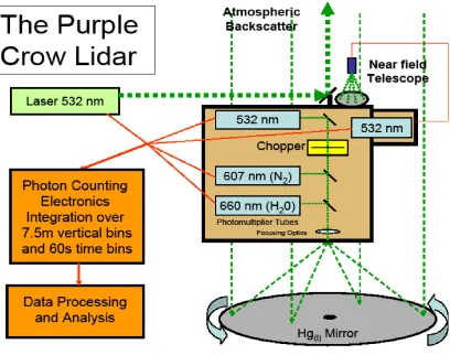
Figure 2.1: PCL schematic diagram containing Hg telescope and receiver system.

both water vapour mixing ratio and Raman temperatures using radiosondes from Detroit and

Buffalo can be found in a paper by Argall et al. [1].

By the summer of 2010 the Delaware Observatory was no longer suitable for PCL and a

new, custom-built observatory was made ready at the Environmental Science Western Field

Station (43.07 N, 81.33 W, 275 m) (Ministry of Natural Resources 1983). The move provided

an opportunity to update and rework PCL and the system received a new, more powerful, laser;

new photomultiplier tubes; new, faster, counting electronics; new optics; an environmentally

friendly geothermal cooling loop for laser temperature stability; and a low dew-point, ultra

clean compressor which supplies air to the liquid mercury telescope. In addition to these

upgrades the new site also offers better seeing conditions and is much closer to campus which

allows for more routine observations. A schematic overview of the system can be found in

(40)

26 Chapter2. LidarInstrumentation

Figure 2.2: Schematic of the Litron LPY-7000 laser head.

2.3 PCL Sub-systems

The Purple Crow Lidar is a mono-static lidar system which was designed and assembled during

the summers of 2010 and 2011 and became fully operational in early 2012. In essence, the

PCL Observatory can be subdivided into three independent sub-systems which will be broadly

labled as: the Transmitter, the Receiver, and the Data Acquisition System. Each of these three

systems will be described separately and the work that has been done in their creation and

calibration will be detailed.

2.3.1 The Transmitter

The Laser head

The PCL uses the second harmonic of a Neodymium: Yttrium-Aluminium-Garnet (Nd:YAG)

solid state laser to produce light at 532 nm. The laser itself is an experimental prototype which

was designed and manufactured by a British company, Litron Lasers. An optical diagram is

shown in Figure 2.2 as a visual reference for the following discussion on the characteristics,

modifications, and operation of this device.

The unseeded, double rod, Gaussian oscillator outputs a 10 ns pulse of coherent 1064 nm

light at a repetition rate of 30 Hz. The measured beam diameter at this point is 8.0±0.5 mm

when run on a fixed Q (time delay) and slightly larger when triggered by an internal Q-switch.

(41)

2.3. PCL Sub-systems 27

with f-numbers ofF−500 andF+572, respectively, before entering the pre-amplifier.

The pre-amplifier contains two laser rods in a deionized water cooled cavity that is

sur-rounded by two flash lamps in a parallel circuit. Separating the flash lamps from the laser rod

cavity are broadband UV filters chosen to protect the laser rods from degradation caused by

UV light in the lamp spectrum.

The pre-amplifier is followed by another set of collimating lenses with f-numbers ofF−200

and F +250, and then by an amplifier which is an identical device to the pre-amplifier. At

this point, the laser beam is still at 1064nm but the laser pulse energy has been increased to

approximately 2500 mJ per pulse with a beam diameter approaching 10 mm. It is important to

note that the position of the oscillator, pre-amplifier, and amplifier are not perfectly co-linear

with the back trajectory of the beam path. The reason for this displaced layout is to introduce a

small angular offset so that any back reflected laser light does not re-enter the previous stage of

the laser and cause damage. To visualize this offset, imagine a very slight, almost indiscernible

by the eye, lightning bolt-shape to the beam path.

After leaving the collimating lenses of the amplifier, the beam travels into the doubler. The

doubler is an oven, in its original design heated to 40◦C which contains a crystal of Potassium

titanyl phosphate (KTiOPO4). The doubling crystal is a solid state non-linear optic which

converts incoming photons at 1064 nm into outgoing 532 nm photons.

Significant work was done, post installation, to modify the oven temperature in an effort to

maintain a constant laser output. The work involved very slowly changing the temperature of

the oven and correcting the phase of the crystal to compensate for thermal drift. This

exper-iment was carried out over 72 hours and required shifts with fellow graduate students Emily

McCullough and Jaya Khana. A new oven temperature of 50◦_{C was selected which allowed}

the laser power to plateau at a stable value. A summary of the results is given in Figure 2.3.

Since running the crystal at such a high temperature is not a good long term solution, Litron

Lasers redesigned and installed a more sophisticated oven which aided in uniform and

(42)

Figure 2.3: Effect of doubler crystal temperature on laser output power.

When the beam exits the doubler chamber the frequency of the light has been changed to

532 nm, the pulse length has been shortened to 8.0 ns, and the new beam diameter is 11±1

mm. Power measurements of the laser output at this point yielded an average pulse energy of

970±50 mJ, an energy density per pulse of∼ 100MW_cm2 and a specified divergence of 0.5 mrad.

The Laser Power Supply and Cooling

Due to the experimental nature of this laser, extensive testing and redesign work was required

for the power supply and coolant systems. The laser assembly was measured to require a 40 A

draw on a 240 V line, a significant amount of power. Given that most lasers have a less than 1%

efficiency in the conversion of electrical energy to light [52] (calculated to be approximately

3% for our system) there is a significant amount of waste heat produced. This heat, calculated

to be approximately 9600 W, must be efficiently removed from the laser head as variations in

the temperature of many optical components like the laser rods and the doubling crystal affect

their lensing properties. The system is designed to operate most efficiently between 18◦C and

(43)

Figure 2.4: Effect of room temperature on laser output power.

Unfortunately, the initial design of both the laser and the PCL Observatory were not able

to dissipate the heat produced in the system at a sufficient rate and the system overheated

after about 30 minutes of use. It was decide that the laser required both a set of cooling fans

mounted into the casing, which would draw air across the outside of the flash lamp casing, and

a geothermal cooling system which couples with the laser’s cooling system and dissipates the

heat in 200 m underground loops. We worked out that the geothermal system was required to

supply 8 L/minute at 30 PSI to the laser power supply which runs a cross-current circulation

into a de-ionized water (DI) loop.

After addressing the concerns regarding the doubler crystal oven temperature, the laser

output power stability, the electrical supply, and the heat dissipation, the laser manifested a

tendency to produce irregular beam shapes. A normal beam shape is a tight Airy diffraction

pattern with an energy density distribution related to the Fourier transform of the aperture. For

a circular aperture of radius, R, equation (2.1) is the transform whereJ1(x) is a Bessel function

(44)

I(θ)= I0

2J1(x)

x2 (2.1)

x=kRsin(θ) (2.2)

This pattern is expected in cases of Fraunhofer, or far field, diffraction. When a beam shape

becomes irregular (in our case the asymmetry begins in the oscillator) there is a tendency to

focus portions of the beam very near to the aperture, or Fresnel diffraction (less than 10 m).

When this process occurs in the laser it develops what are called hot spots which are regions in

the beam where the energy density spikes up due to intra-beam focusing.

When these hot spots occur over optics in the beam path they act to deposit energy into

the material at a rate which is faster than the optic coating or underlying glass can thermally

dissipate. At this point, chemistry becomes an issue as the specialized coatings on the optics

oxidizes, rendering the component useless. As a relative measure of the intensity of the hot

spots, the average central energy fluence of the laser is 110±10 MW_cm2 and the hot spot was able

to burn through optical coating rated at 500 MW_cm2.

The beam hot spots in our system burned through several of the internal optics in the laser

head, scorched the ends of the laser rods, burned the coatings offof the PCL beam expander

(discussed in the next section), and made holes in a few of our old 532 nm laser line mirrors.

After replacing all the damaged components, the laser technicians from Litron and I developed

a procedure to damp out the hot spots by deliberately misaligning the laser and reducing the

overall output power.

There are two main ways to modulate laser power: the first and most simple way is to

change the voltage that the system puts across the flash lamps. Thinking back to the laser

chamber, we see a simple system where the potential across the lamps induce a greater

re-sponse, which pumps more energy into the laser rods, which in turn increases the total laser

(45)

Figure 2.5: The output power of the laser can be modulated by varying the delay between triggering of the Oscillator (blue), Pre-amplifier (magenta), and Amplifier (yellow). The time delay of the emitted pulse is shown in green. [31]

maintaining a consistent flash as the bulbs degrade and discolour over time.

The second part of the method for modulating the laser output is to adjust the pulse delay

across the laser head. Referring back to Figure 2.2, we see that each of the three pumping

chambers (the oscillator, pre-amplifier, and amplifier) and the Q-switch are precisely positioned

in the laser head. Given that light travels at the speed of light,c, and that the laser must output

30 pulses per second, it is important that each of the pumping chambers and the Q-switch are

properly synchronized. When a pulse originates in the oscillator and then travels to the

pre-amplifier the delay on the pre-pre-amplifier must be set so that it adds energy to the pulse in phase.

The same must hold with the pulses coming to the amplifier and Q-switch. Figure 2.5 is from

the laser manual and gives an illustrative picture of this delay between pulse generation and

pulse output across the system [31]. By introducing an offset in the pulse delay between the

Q-switch and the outgoing pulse, the energy of the system is damped and the change in the

lasing temperature of the rods helps to minimize the hot spots. To compensate for changing the

(46)

of the doubling crystal. Dr. Steve Argall built a small switch controlled potentiometer which

allows me to change the delay in real time while the system is operational. Without this device

it would be too dangerous to conduct this procedure. Balancing the timing delay, voltage, and

crystal angle has allowed me to maintain a relatively constant output of 600 mJ per pulse on the

system. This reduced, but stable, output was sufficient for PCL to participate in a calibration

experiment with NASA GFSCs ALVICE lidar (described in Chapter 4). It is important to note

that this quick fix has a number of problems which must be addressed:

1) The hot spots are only minimized, not eliminated. They will likely continue to degrade

the internal optics of the laser over time.

2) The procedure to balance the pulse delay, voltage and crystal phase is a very delicate and

non-trivial procedure where experience with this particular laser and intuition are valuable.

When the potential or pulse delay is changed the local heating on the laser rods also changes

which alters their lensing properties. If care is not taken in this procedure the flash lamps can

explode, the beam shape can become distorted, or the doubler crystal can burn.

3) There is a finite length of time that this method can be employed before the corrections

to the pulse delay become of the order of the pulse separation. Fortunately, the laser has gone

back to the Litron factory for a redesign and rebuild of the oscillator which should hopefully

correct the beam defect.

The Beam Expander

After the beam leaves the laser head, it passes through a pair of lenses to expand the beam

in an effort to minimize the beam divergence of 0.5 mrad. The original beam expander was

designed by Dr. Argall and was composed of a pair of lenses mounted in a set of optical stands.

Unfortunately, these optics were destroyed by hot spots in the beam. Upon closer examination

of the outgoing laser beam it was discovered that the beam divergence was larger than specified

by the manufacturer.

(47)

Figure 2.6: Schematic of beam expander. [60]

was purchased from Special Optics the specifications of which are given in figure 2.6. This

new set up expands the beam from a diameter of 12 mm with a divergence greater than 0.5

mrad to a 600 mm beam with a divergence less than 87 µrad. An ´etalon was used to ensure

proper collimation of the outgoing laser beam.

Beam expanders work to reduce the beam divergence in the far field by increasing the final

aperture size of the terminal optic. Assume a setup as shown in figure 2.7 whereD0is the optic

aperture or beam waist,θis the beam divergence,xis a suitably far distance from the aperture

such that near field optical effects are no longer dominant, andD(x) is the diameter of the beam

at distance x. Diffraction is the spreading of light which is emitted from a finite source and it

makes beam collimation impossible. As the laser beam exits the aperture secondary waves

arise from the characteristics of the edges of the optic. These secondary waves interfere with

(48)

Figure 2.7: Depiction of far field divergence from a laser aperture or terminal optic.

The spreading of the beam can be expressed by equation (2.3) where

D(x)= D0

s

1+ λx πS2₀

!2

(2.3)

S(x)≈ λx

πS0

. (2.4)

θ= S(x)

x ≈

λ πS0

(2.5)

λis the laser wave length. If _πλ_Sx2 0

>>1, which is the case for the far field where xcan be large,

then equation (2.3) can be approximated by equation (2.4). Then using some trigonometry,

the divergence angle θ can be approximated by equation (2.5). As can be seen, there is an

inverse relationship between the beam width and the far field divergence, therefore expanding

the Gaussian laser beam through a Galilean telescope acts to tighten the beam. [18] Having a

small beam size is important for lidar studies and will be discussed later in this chapter.

The Optical Path

The collimated beam travels through 13.418 m and reflects offthree 2.5 inch laser line mirrors

(49)

Figure 2.8: Original blueprint for the PCL optical transmission path.

on top of the detector box, is a commercial motorized mirror mount. This mount is computer

controlled to tilt the laser beam in the sky for optimal alignment.

2.3.2 The Receiver

The Liquid Mercury Telescope

The primary receiving optic for the PCL is a mirror made from a rotating dish of liquid mercury.

The initial design of the liquid mercury telescope was done by Prof. Ermanno Borra and

colleagues at the Universit´e Laval [7] and [8] and it was built with the expertise of Prof. P.

Hickson (UBC). The advantage to using a liquid mirror telescope in lidar studies is that it

allows for a relatively large, relatively inexpensive, alternative to a glass mirror. An added

Multi-Sensor Calibration and Validation of the UWO-PCL Water Vapour Lidar

Scholarship@Western

Scholarship@Western

Multi-Sensor Calibration and Validation of the UWO-PCL Water

Multi-Sensor Calibration and Validation of the UWO-PCL Water

Vapour Lidar

Vapour Lidar

MULTI-SENSOR CALIBRATION AND VALIDATION OF THE UWO-PCL

WATER VAPOUR LIDAR

(Spine title: Calibration of the PCL Water Vapour Lidar)

(Thesis format: Monograph)

by

Robin Wing

Graduate Program in Physics and Astronomy

A thesis submitted in partial fulfillment

of the requirements for the degree of

Masters of Science

The School of Graduate and Postdoctoral Studies

The University of Western Ontario

London, Ontario, Canada

c

THE UNIVERSITY OF WESTERN ONTARIO

School of Graduate and Postdoctoral Studies

CERTIFICATE OF EXAMINATION

Acknowlegements

Abstract

Contents

List of Figures

List of Tables

List of Appendices

Chapter 1

A Review of Some Atmospheric Concepts

1.1

Introduction

1.2

Atmosphere Pressure for an Isothermal Atmosphere

1.3

Atmospheric Composition

1.4

Temperature Structure

1.5

Troposphere

1.6

Stratosphere

1.7

Water Vapour in the Atmosphere

1.7.1

Qualitative Discussion

1.7.2

Quantitative Discussion

1.7.3

Saturation Vapour Pressure as Applied to the Atmosphere

1.8

Atmospheric Scattering

1.8.1

Mie Scattering

1.8.2

Rayleigh Scattering

1.8.3

Raman Scattering

Chapter 2

Lidar Instrumentation

2.1

Introduction

2.2

The Purple Crow Lidar History

2.3

PCL Sub-systems

2.3.1

The Transmitter

2.3.2

The Receiver